Download
1 / 33
340 likes | 590 Vues
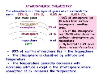
Fundamentals of atmospheric chemistry modeling. Types of models Chemical Solvers The Continuity Equation Emissions Parameterisations for Deposition and Lightning. What is a model?.

E N D
Fundamentals of atmospheric chemistry modeling Types of models Chemical Solvers The Continuity Equation Emissions Parameterisations for Deposition and Lightning
What is a model? A model „simulates“ reality, i.e. it describes a certain aspect of the world in a simplified and understandable manner. Models can be used to predict things (e.g. the architectural model tells you how a building might look like), or they are used to perform „what if“ scenarios, which are often not feasible in the real world. Since models contain what we know, comparing simulation results with reality (measurements) often helps to elucidate areas where our understanding is weak.
Types of (atmosphere) models • box (compartment) models:understand the principles of feedback cycles • 0D (point) models:detailed analysis of the chemical tendencies for a given situation; analysis of sensitivities • 1D column models:development of parameterisations • 1D lagrangian (trajectory) models:transport studies • 2D (eulerian) models:zonal mean state of the atmosphere (often in stratosphere) • 3D (eulerian) models:detailed description of several processes in time and space
6 TgC/yr fossil fuelcombustion Atmosphere 615 TgC 90 60 61 92 Land Biosphere Surface Ocean 730 TgC 840 TgC 0.2 0.2 Sediments 90,000,000 TgC Box models Example: A very simplified box model of the global carbon cycle
NOx O3 HO2 0D (point) models Idea: investigate the chemistry in an „air parcel“ without regarding advection or diffusion processes Long-lived compounds treated as boundary conditions; often run as „steady state“ simulation Advantage: computationally very fast, allows for comprehensive chemical mechanism, Monte Carlo simulations, etc. Disadvantage: does not take transport into account
Quasi steady state approximation If the loss of a chemical species is much faster than its production (and fast compared to the length of a day), it is generally a reasonable assumption to assume that it is in „dynamic steady state“, i.e. dX/dt = 0. Example: thus This approach has been used for the „Quasi Steady State Model“, which you can find on my web page.
Validity of QSSA reasonable good
Emissions NO +O3, +HO2 +h NO2 +OH, deposition Chemical Families A „trick“ to make the QSSA approach work for longer-lived species as well is the definition of chemical „families“: Species are grouped together so that the fast reactions don‘t change the group concentration. Example: NOx = NO + NO2
Solving chemical equations numerically Disregarding emissions and deposition (which are treated elsewhere), the differential equations for the reactions between species take the form: where P and L are functions of µ, T, p, etc.. For most reactions, the lossrate is proportional to µi, so that one can write L = ·µi(exceptions: radical self reactions, e.g. HO2+HO2) The chemical lifetime of species i is then given as = P/. In the atmosphere, the lifetimes vary from microseconds to years. Therefore,the set of reaction equations is called „stiff“.
Solving chemical equations numerically (2) Because of the coupling between the chemical equations (loss of one species is production of another one), the set of differential equations describing the reactions must be solved numerically, i.e. with a discrete time step. The concentration of species i at time t is then given as: (Taylor expansion) Numerical solvers differ in the number of terms they carry, the time step for which the derivatives are evaluated, and the numerical methods for solving the matrix equations.
Explicit solvers When derivatives are evaluated only from concentrations of the previous time step(s), the solution is called „explicit“. Example: Forward Euler scheme This is a first order approximation, where all derivatives are evaluated for timestep t-1. Advantage: exactly mass conserving Disadvantage: numerically unstable if time step exceeds time of fastest reaction. I.e. a time step of 10-4 s is needed for atmospheric photochemistry; this becomes computationally unfeasible.
Semiimplicit solvers If at least some of the derivatives are evaluated at the time step t, the method is called „implicit“ (or semiimplicit). Example: Backward Euler scheme As in the forward Euler scheme, all derivatives are evaluated at t-1, except those for species i. This results in an equation for µi: Advantage: stable and positive definite Disadvantage: not exactly mass conserving, because the linearized rates differ slightly:
Multistep solvers If the backward Euler method is applied recursively until convergence is achieved for all species, the errors become neglible. This method is used in MOZART. Other multistep methods include the „Multistep implicit explicit“ solution, where explicit and implicit steps are alternated, or the Gear method, which involves higher-order terms, and is computationally more expensive (for details see Jacobson, Fundamentals of Atmospheric Modeling).
Lagrangian models Lagrangian (or trajectory) models are in fact 3-dimensional in that they take account of the horizontal and vertical transport of an air parcel. „We define a transition probability density Q(X0,t0|X,t), such that the probability that the fluid element will have moved to within volume (dx,dy,dz) centered at location X at time t is Q(X0,t0|X,t) dx dy dz.“ (Jacob, 1999) t0 t While this approach implicitely accounts for small-scale processes like diffusion or convection, it has disadvantages, because it neglects mixing of air parcels, and the quantity Q is not directly observable. One way of using the lagrangian technique efficiently is the particle model, where Q is approximated by a large number of point-like particles (~10000), and a trajectory for each particle is computed using stochastic methods to simulate diffusion. Example: Stohl et al., 2000.
2-dimensional models This type of model has been used primarily in stratospheric applications, because there the assumption of zonally homogeneous fields is closer to reality than in the troposphere, where continents and emission sources produce large meridional gradients. Example: Daily averaged NOx mixing ratio for 90hPa (left) and 850 hPa (right) from a 3-dimensional MOZART simulation
3-dimensional eulerian models This model type represents the most comprehensive, but also computationally most expensive type of models. The earth‘ atmosphere is divided into thousands of „grid boxes“ of more or less regular shape. Examples: Grid box boundaries over Europe for a „T21“ grid with 64x32 boxes globally (left), and a 1°x1° grid (right)
Orography Depending on the model resolution, the landscape will be resolved with more or less detail. Example: The altitude of the Alps is about 350 m in the T21 resolution (left)! At 1°x1° (right) the Alps extend to altitudes of about 1.2 km. Obviously, this will impact the flow of air! Note that even a 1x1 grid is far from sufficient to resolve valley flow.
... =0.985 =1 Vertical Coordinate System Vertical coorinates are usually given either as constant pressure levels (p), terrain following „“ levels, „hybrid“ coordinates (a mixture between p and ). Sometimes,z coordinates (alitudes) are used. The definition of coordinates is: I.e. the actual pressure of a specific model level depends on the surface pressure for this grid box (and changes with time). The use of coordinates facilitates the formulation of the (physical) conservation equations (see Hartmann, 1994). Some models number the levels from top to bottom, in others it is bottom-top. Hybrid levels are defined as pi = A·p0+B · ps, where p0 is a constant reference pressure (100000 Pa).
The continuity equation Consider a volume element (dx dy dz) in a fixed cartesian system. Then the (one-dimensional) net flow of mass through the box is given as: left boundary right boundary dz dx dy For three dimensions, this becomes: The accumulation rate of mass in the box (local density change) must equal the net inflow into the box.
Applying the vector identity and the relationship yields the velocity divergence form of the continuity equation: The continuity equation (2) A similar continuity equation holds for the mass of a tracer i: The terms on the right hand side denote the (photo)chemical production and loss, emissions, and deposition of the tracer.
Turbulence Separating the large-scale (synoptic) motion from the small-scale turbulence yields: and e.g. Then the (one-dimensional) continuity equation becomes: A scale analysis shows that only are relevant. The diffusive transport can then be expressed as: with K being the eddy diffusivity constant. This is the so-called „Large Eddy approximation“.
Operator splitting One of the great „sins“ in modeling is the assumption, that the individual processes can be treated sequentially, i.e. is assumed to be equivalent to: Each of the terms on the right hand side is then solved by its own „operator“. Experience shows that the solution is stable and reasonable if the time step is short enough.
Advection Courant-Friedrichs-Lewy (CFL) condition: Meaning: the time step must be small enough, so that an air parcel does not pass through more than 1 grid box during one time step. • A good advection scheme should be: • mass conserving • shape preserving • positive definite • local • fast • In today‘s models, typically lagrangian or semi-lagrangian transport schemes are used.
arrivalpoint (x,t) (x0,t0) departurepoint Semi-Lagrangian transport In semi-lagrangian transport schemes, a backward trajectory is computed for each corner point of a grid cell. The new mixing ratio of species i is then computed by interpolation („remapping“) of the concentration field of timestep t0 onto the model grid at timestep t.
Emissions In current models, emissions are typically specified as monthly mean mass fluxes. These are read from file and interpolated to time t. The compilation of emissions inventories is a labour-intensive task, and these inventories still constitute one of the major uncertainties in modeling. Today, first attempts have been made to estimate emissions based on satellite and in-situ observations and using „inverse“ models.
Emissions (2) Typical categories of „bottom-up“ emissions inventories include: • fossil fuel combustion • biofuel combustion • vegetation fires • biogenic emissions (plants and soils) • volcanic emissions • oceanic emissions • agricultural emissions (incl. fertilisation) etc.
Vegetation fire emissions aka „biomass burning“ Classic approach: use forest fire statistics, observations of „fire return intervals“, and average parameters for fuel load and burning efficiency, and derive a climatological inventory. Disadvantage: vegetation fires occur episodically and exhibit a large interannual variability. New approach: Use satellite observations of burned areas and measured or model-derived parameters for the available biomass and the fire behaviour.
The Global Wildfire Emission Model (GWEM) J. Hoelzemann area burnt combustionefficiency fuelload emissionfactor
(Dry) Deposition Transport of gaseous and particulate species from the atmosphere onto surfaces in the absence of precipitation Controlling factors: atmospheric turbulence, chemical properties of species, and nature of the surface Deposition flux: vd: deposition velocity C: concentration of species at reference height (~10 m)
atmosphere Ra Rb Rc surface Resistance analog Ra = aerodynamic res. Rb = quasi laminar boundary layer resistance Rc = canopy resistance Seinfeld & Pandis, 1998
Cloud Water chemical reactions evaporation evaporation nucleation dissolution rain formation particlesin air gaseous speciesin air reactions below-cloudscavenging below-cloudscavenging Rain, snow chemical reactions evaporation evaporation interception Wet deposition Wet deposition after Seinfeld&Pandis, 1998
Bibliography • Holton, J.R., An Introduction to Dynamic Meteorology, Academic Press, San Diego, ..., 31992. • Peixoto, J.P., and Oort, A.H., Physics of Climate, Springer, New York, 1992. • Jacobson, M.Z., Fundamentals of atmospheric modeling, Cambridge University Press, Cambridge, New York, 1999. • Brasseur, G.P., Orlando, J.J., and Tyndall, G.S., Atmospheric Chemkistry and Global Change, Oxford University Press, Oxford, New York, 1999. • Hartmann, D.L., Global Physical Climatology, Academic Press, San Diego, ..., 1994. • Durran, D.R., Numerical Methods for Wave Equations in Geophysical Fluid Dynamics, Springer, New York, ..., 1998.