Download

1 / 40
400 likes | 475 Vues
The ENSEMBLES high-resolution gridded daily observed dataset. Malcolm Haylock, Phil Jones, Climatic Research Unit, UK WP5.1 team: KNMI, MeteoSwiss, Oxford University. Outline. The gridded dataset: who, why, when and what? The station network Interpolation method comparison

E N D
The ENSEMBLES high-resolution gridded daily observed dataset Malcolm Haylock, Phil Jones, Climatic Research Unit, UK WP5.1 team: KNMI, MeteoSwiss, Oxford University
Outline • The gridded dataset: who, why, when and what? • The station network • Interpolation • method comparison • two-step interpolation of monthly and daily data • kriging and extremes • Point vs interpolated extremes • implication for RCM validation • Uncertainty • Then finally some analyses comparing with GCM simulations from RT2B with ERA-40 forcing
The dataset… • Who: • Four groups in WP5.1 • KNMI: data gathering and data quality and homogenisation • MeteoSwiss: homogeneity of temperature data • UEA and Oxford: interpolation • Why • Validation of RCMs • Climate change studies • Impacts models • Many data providers do not allow distribution of station data
…The dataset… • When • Daily 1950-2006 • Available now from ENSEMBLES web site plus ECA&D • Two papers submitted to JGR, one on the comparison of methods, and one on the final gridded dataset with the chosen methods , which differ by variable • What • Five variables • precipitation • mean, minimum and maximum temperature • mean sea level pressure (early 2008) • Europe • 0.250 and 0.50 CRU grids • common RCM rotated-pole grid0.220 and 0.440 rotated pole (-162.00, 39.250)
Tmean Stations 1231
Interpolation • Need to match observations to model grid for direct comparison • Therefore need to estimate observations at “unsampled” locations • Compare several methods to find most accurate at reproducing observations in a cross validation exercise – see more in Nynke Hofstra’s presentation tomorrow • Largest QC problem is that date of observations do not match – day is day when values occurred, but sometimes it is day when measured
Interpolation Methods • Natural neighbour interpolation • Angular distance weighting • Thin-plate splines • 2-D and 3-D • Kriging • 2-D and 3-D • 4-D Regression • lat, lon, elevation and distance to coast • Conditional Interpolation – important for precipitation
Cross Validation • . For each station, interpolate to that station using its neighbours and compare with the observed value. • Repeat for all days. • Do for monthly averages and daily anomalies Daily precipitation (% of monthly total) compound relative error (cre) = rms / σ critical success index (csi) = hits/(false alarm+hits+misses)
Cross Validation Daily pressure (anomaly from monthly mean) precip: 2-D kriging with separate occurrence model pressure: 2-D kriging Tmean, Tmin, Tmax: 3-D kriging Daily Tmean (anomaly from monthly mean)
Interpolation methodology • Grid monthly means using 2-D (pressure) and 3-D (temp and precipitation) thin-plate splines • Determined to be the best method using cross validation • Grid daily anomalies using kriging • Combine the interpolated monthly means and the interpolated anomalies as well as their uncertainty • Create a high resolution master grid (10km rotated-pole grid) and do area averaging to create different coarser resolution products.
Kriging and extremes • Kriging estimates the mean and variance of the distribution at unsampled locations • The best guess is the mean but extremes are usually a combination of a high local signal superimposed on a high background state • Therefore kriging will tend to underestimate extremes and produce results similar to the area mean
Precipitation interpolation extremes reduction factor 2yr 5yr 10yr 50% 75% 90% 95% 99%
Tmax interpolation extremes -reduction in anomaly 50% 75% 90% 95% 99% 2yr 5yr 10yr
Precipitation Extremes Gridded Extremes Extremes of Gridded precipitation 10-year return period
Uncertainty • Interpolation uncertainty only
Conclusions • We have created a European daily dataset very much improved over previous products, with a detailed comparison of interpolation methods • Kriging gives the best estimate of a point source, but when the interpolated grid (25km) is smaller than the average separation (45km for precipitation), the interpolated point will be more an area average • Therefore validation of RCMs using the gridded data assumes the RCMs represent area-averages • Kriging can be extended to produce more realistic “simulations” of point precipitation at unsampled locations, with a better estimate of uncertainty of the extremes, but this is computationally very expensive
ENSEMBLES WP5.4 and ETCCDI Meeting – KNMI De Bilt – 13-16 May 2008 Extremes of temperature and precipitation as seen in the daily gridded datasets for surface climate variables (D5.18 – Haylock et al.) and in the RCM model output from the (RT3) 40-year experiments driven by ERA-40 reanalysis data Phil Jones and David Lister – Climatic Research Unit
Gridded Data • Available on ENSEMBLES web site • Two papers submitted to JGR • One on a comparison of gridding techniques (Hofstra et al.) • One on the final gridded dataset (Haylock et al.) • A simple comparison shown here
The location and period of coverage of station-series which went into the interpolation/gridding exercise
Extreme Measures • Trends of mean maximum and minimum temperatures • Trends of 5th percentile of Tn • Trends of 95th percentile of Tx • Compare gridded trends with station trends • Trends patterns over various periods
Testing of extreme values in a fairly flat part of the region covered by the observed grids – Lubny, Ukraine
Trends (°C/decade) in the (gridded/observed) 05th percentile Tmin. series – 1950-2006
Trends (°C/decade) in the CRU 0.5° grids (CRU TS3.0) Tmin. series – 1950-2006
Trends (°C/decade) in the (gridded/observed) 95th percentile Tmax. series – 1950-2006
Trends (°C/decade) in the (gridded/observed) 05th percentile Tmin. series – 1961-2006
Trends (°C/decade) in the (gridded/observed) 95th percentile Tmax. series – 1961-2006
Tn05 – histogram of differences compared to gridded observations
Tx95 – histogram of differences compared to gridded observations