Download
1 / 38
620 likes | 1.29k Vues
9. Third-order Nonlinearities: Four-wave mixing. Third-harmonic generation Induced gratings Phase conjugation Nonlinear refractive index Self-focusing Self-phase modulation Continuum generation. THG Medium. w. 3 w. Third-harmonic generation. We must now cube the input field:.

E N D
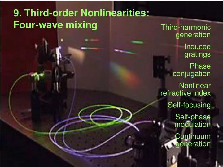
9. Third-order Nonlinearities: Four-wave mixing Third-harmonic generation Induced gratings Phase conjugation Nonlinear refractive index Self-focusing Self-phase modulation Continuum generation
THG Medium w 3w Third-harmonic generation We must now cube the input field: Third-harmonic generation is weaker than second-harmonic and sum-frequency generation, so the third harmonic is usually generated using SHG followed by SFG, rather than by direct THG.
Signal #1 THG medium w w w w w w Signal #2 Noncollinear Third-Harmonic Generation We can also allow two different input beams, whose frequencies can be different. So in addition to generating the third harmonic of each input beam, the medium will generate interesting sum frequencies.
Signal #1 w w Nonlinear medium w w w w Signal #2 Third-order difference-frequency generation: Self-diffraction Consider some of the difference-frequency terms:
Signal Sample medium w w w The excite-probe geometry One field can contribute two factors, one E and the other E*. This will involve both adding and subtracting the frequency and its k-vector. This effect is automatically phase-matched! The excite-probe beam geometry has many applications, especially to ultrafast spectroscopy. The signal beam can be difficult to separate from the input beam, E1, however.
Wave plate yielding 45˚ polarization Signal w Nonlinear medium w w The input beam is the signal beam direction is rejected by polarizer! Polarization gating Here field #2 contributes two factors, one E and the other E*. But one is vertically polarized, while the other is horizontally polarized. This yields a signal beam that’s orthogonally polarized to the input beam E1. If E1 is horizontally polarized, the signal will be vertically polarized: This arrangement is also automatically phase-matched. It’s also referred to as polarization spectroscopy due to its many uses in both ultrafast and frequency-domain spectroscopy.
Many nonlinear-optical effects can beconsidered as induced gratings. x x x x x The irradiance of two crossed beams is sinusoidal, inducing a sinusoidal absorption or refractive index in the medium––a diffraction grating! An induced grating results from the cross term in the irradiance: Time-independent fringes
x Diffraction off an induced grating A third beam will then diffract into a different direction. This results in a beam that’s the product of E1, E2*, and E3: This is just a generic four-wave-mixing effect.
qex Nonlinear medium wex1 z wex2 qsig wpr qpr wsig=wpr Diffracted signal Induced gratings Assume: but Phase-matching condition: The diffracted beam has the same frequency and k-vector magnitude as the probe beam, but its direction will be different.
qex x wex z wex qsig wpr qpr Phase-matching induced gratings Phase-matching condition: The minus sign is just the excite-probe effect. z-component: x-component: The “Bragg Condition”
Nonlinear medium w1 w2 w3 w1 w2 +w3 Diffracted signal Induced gratingswith different frequencies This effect is called “non-degenerate four-wave mixing.” In this case, the intensity fringes sweep through the medium: a moving grating. Phase-matching condition: The set of possible beam geometries is complex. See my thesis!
Induced gratings with plane waves and more complex beams (of the same frequency) A plane wave and a slightly distorted wave A plane wave and a very distorted wave Two plane waves A plane wave and a slightly distorted wave All such induced gratings will diffract a plane wave, reproducing the distorted wave: E2 and E3 are plane waves.
Holography is an induced-grating process. One of the write beams has a complex spatial pattern that is the image. Different incidence angles correspond to different fringe spacings, so different views of the object are stored as different fringe spacings. A third beam (a plane wave) diffracts off the grating, acquiring the image information. In addition, different fringe spacings yield different diffraction angles––hence 3D! The light phase stores the angular info.
Phase conjugation When a nonlinear-optical effect produces a light wave proportional to E*, the process is called a phase-conjugation process. Phase conjugators can cancel out aberrations. A normal mirror leaves the sign of the phase unchanged A phase-conjugate mirrorreverses the sign of the phase The second traversal through the medium cancels out the phase distortion caused by the first pass!
Phase Conjugation = Time Reversal A light wave is given by: If we can phase-conjugate the spatial part, we have: Thus phase conjugation produces a time-reversed beam!
Consider only processes with three input frequencies and an output frequency that are identical. Degenerate Four-Wave Mixing Because the k-vectors can have different directions, we’ll distinguish between them (as well as the fields): Degenerate four-wave mixing gives rise to an amazing variety of interesting effects. Some are desirable. Some are not. Some are desirable some of the time and not the rest of the time.
If just one beam is involved, all the k-vectors will be the same, as will the fields: Single-Field Degenerate Four-Wave Mixing So the polarization becomes: Single-field degenerate four-wave mixing gives rise to “self” effects. These include: Self-phase modulation Self-focusing (whole-beam and small-scale) Both of these effects participate in the generation of ultrashort pulses!
Degenerate 4WM means a nonlinearrefractive index. Recall the inhomogeneous wave equation: and the polarization envelope (the linear and nonlinear terms): Substituting the polarization into the wave equation (assuming slow variation in the envelope of E compared to 1/w): since So the refractive index is:
since: The refractive index in the presence of linear and nonlinear polarizations: Nonlinear refractive index (cont’d) Now, the usual refractive index (which we’ll call n0) is: So: Assume that the nonlinear term << n0: So: Usually we define a “nonlinear refractive index”, n2:
The nonlinear refractive index magnitude and response time A variety of effects give rise to a nonlinear refractive index. Those that yield a large n2 typically have a slow response. Thermal effects yield a huge nonlinear refractive index through thermal expansion due to energy deposition, but they are very very slow. As a result, most media, including even Chinese tea, have nonlinear refractive indices!
The nonlinear refractive index, , causes beams to self-focus. Whole-Beam Self-Focusing If the beam has a spatial Gaussian intensity profile, then any nonlinear medium will have a spatial refractive index profile that is also Gaussian: Near beam center: The phase delay vs. radial co-ordinate will be: This is precisely the behavior of a lens! But one whose focal power scales with the intensity.
Intensity Position If the beam has variations in intensity across its profile, it undergoes small-scale self-focusing. Small-Scale Self-Focusing Each tiny bump in the beam undergoes its own separate self-focusing, yielding a tightly focused spot inside the beam, called a “filament.” Such filaments grow exponentially with distance. And they grow from quantum noise in the beam, which is always there. As a result, an intense beam cannot propagate through any medium without degenerating into a mass of tiny highly intense filaments, which, even worse, badly damage the medium.
The self-phase-modulated pulse develops a phase vs. time proportional to the input pulse intensity vs. time. Self-Phase Modulation & Continuum Generation Pulse intensity vs. time The further the pulse travels, the more modulation occurs. That is: A flat phase vs. time yields the narrowest spectrum. If we assume the pulse starts with a flat phase, then SPM broadens the spectrum. This is not a small effect! A total phase variation of hundreds can occur! A broad spectrum generated in this manner is called a “Continuum.”
The instantaneous frequency vs. time in SPM A 10-fs, 800-nm pulse that’s experienced self-phase modulation with a peak magnitude of 1 radian.
Self-phase-modulated pulse in the frequency domain The same 10-fs, 800-nm pulse that’s experienced self-phase modulation with a peak magnitude of 1 radian. It’s easy to achieve many radians for phase delay, however.
A highly self-phase-modulated pulse A 10-fs, 800-nm pulse that’s experienced self-phase modulation with a peak magnitude of 10 radians Note that the spectrum has broadened significantly. When SPM is very strong, it broadens the spectrum a lot. We call this effect continuum generation.
Experimental Continuum spectrum in a fiber Continua created by propagating 500-fs 625nm pulses through 30 cm of single-mode fiber. Low Energy Medium Energy High Energy The Supercontinuum Laser Source, Alfano, ed. Broadest spectrum occurs for highest energy.
Continuum Generation Simulations Instantaneously responding n2; maximum SPM phase = 72π radians Input Intensity vs. time (and hence output phase vs. time) The Supercontinuum Laser Source, Alfano, ed. Original spectrum is negligible in width compared to the output spectrum. Output spectrum: w Oscillations occur in spectrum because all frequencies occur twice and interfere, except for inflection points, which yield maximum and minimum frequencies.
Continuum Generation Simulation Noninstantaneously responding n2; maximum SPM phase = 72π radians Output phase vs. time (≠ input intensity vs. time, due to slow response) Output spectrum: Asymmetry in phase vs. time yields asymmetry in spectrum. The Supercontinuum Laser Source, Alfano, ed.
Input wavelength Experimental Continuum Spectra 625-nm (70 fs and 2 ps) pulses in Xe gas p = 15 & 40 atm L = 90 cm The Supercontinuum Laser Source, Alfano, ed. Data taken by Corkum, et al.
Ultraviolet continuum 4-mJ 160-fs 308-nm pulses in 40 atm of Ar; 60-cm long cell. Lens focal length = 50 cm. Good quality output mode. The Supercontinuum Laser Source, Alfano, ed.
UV Continuum in Air! 308 nm input pulse; weak focusing with a 1-m lens. The Supercontinuum Laser Source, Alfano, ed. Continuum is limited when GVD causes the pulse to spread, reducing the intensity.
Continuum Generation:Good news and bad news Good news: It broadens the spectrum, offering a useful ultrafast white-light source and possible pulse shortening. Bad news: Pulse shapes are uncontrollable. Theory is struggling to keep up with experiments. In a bulk medium, spectral broadening is not really that great— you need a log scale to see it… In a bulk medium, continuum can be high-energy, but it’s a mess spatially. In a fiber, continuum is clean, but it’s low-energy. In hollow fibers, things get somewhat better. Main problem: dispersion spreads the pulse, limiting the spectral broadening.
The continuum from microstructure optical fiber is ultrabroadband. Cross section of the microstructure fiber. The spectrum extends from ~400 to ~1500 nm and is relatively flat (when averaged over time). This continuum was created using unamplified Ti:Sapphire pulses. J.K. Ranka, R.S. Windeler, and A.J. Stentz, Opt. Lett. Vol. 25, pp. 25-27, 2000
Other third-order nonlinear-optical effects Two-photon absorption Raman scattering