Download
1 / 21
1.18k likes | 2.98k Vues
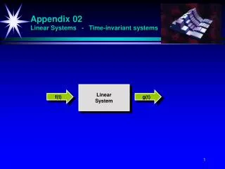
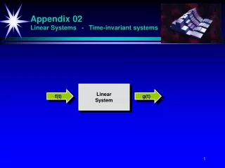
Linear Time Invariant Systems. Definitions A linear system may be defined as one which obeys the Principle of Superposition , which may be stated as follows:

E N D
Linear Time Invariant Systems Definitions • A linear system may be defined as one which obeys the Principle of Superposition, which may be stated as follows: If an input consisting the sum of a number of signals is applied to a linear system, then the output is the sum, or superposition, of the system’s responses to each signal considered separately. • A time-invariant system is one whose properties do not vary with time. The only effect of a time-shift on an input signal to the system is a corresponding time-shift in its output. • A causal system is one if the output signal depends only on present and/or previous values of the input. In other words all real time systems must be causal; but if data were stored and subsequently processed at a later date, it need not be causal.
The Unit Impulse Response • The unit impulse is a single vertical line of zero width and a height of 1. • This is also sometimes known as the Kronecker delta function • d[n] is the symbol given to the line where d means infinitely small. • n is the sampling period • A shifted impulse such as d[n – 2] is the line shifted to the right 2 sampling periods.
Now consider the following signal: x[n] = 2d[n ] + 4d[n – 1] + 6d[n – 2] + 4d[n – 3] + 2d[n – 4] Hence any sequence can be represented by the equation: = + x[-1]d[n + 1] + x[0]d[n] + x[1]d[n - 1] + x[2]d[n - 2] +……. x[k] is the height of each impulse, frequently known as the coefficient. d [n - k] is the time slot
Impulse Response • When the input to an FIR filter is a unit impulse sequence, x[n] = d[n], the output is known as the unit impulse response, which is normally donated as h[n]. A single impulse input yields the system’s impulse response
A scaled impulse input yields a scaled response, due to the scaling property of the system's linearity.
This now demonstrates the additivity portion of the linearity property of the system to complete the picture. Since any discrete-time signal is just a sum of scaled and shifted discrete-time impulses, we can find the output from knowing the input and the impulse response
Convolution • Convolution is a weighted moving average with one signal flipped back to front: • The general expression for an FIR filter’s output is:- A tabulated version of convolution h[0]x[n] = x[0] * h[0] + x[1] * h[0] + x[2] * h[0] + x[3] * h[0] + x[4] * h[0] h[0]x[n] = 2 * 3 + 4 * 3 + 6 * 3 + 4 * 3 + 2 * 3 h[0]x[n] = 6 + 12 + 18 + 12 + 6
FIR Filter y(n) Where Z-n is a delay of one sampling period aR is the coefficient (gain/attenuation of impulse S is the symbol for summation (adding)
Now the following share prices were obtained from a weeks trading
x(0) = 20 x(-1) = 0 x(-2) = 0 Performing the multiplications and additions gives: y(0) = 0.25 x 20 + 0.5 x 0 + 0.25 x 0 = 5
For Tuesday x(1) = 20 x(0) = 20 x(-1) = 0 It follows that: y(1) = 0.25 x 20 + 0.5 x 20 + 0.25 x 0 = 15 For Wednesday x(2) = 20 x(1) = 20 x(0) = 20 Giving: y(2) = 0.25 x 20 + 0.5 x 20 + 0.25 x 20 = 20 For Thursday x(3) = 12 x(2) = 20 x(1) = 20 Giving y(3) = 0.25 x 12 + 0.5 x 20 + 0.25 x 20 = 18
The input impulse pulse train The impulse response of the filter h(n)
Steps, Impulses and Ramps • The unit step function u[n] is defined as: u[n] = 0, n < 0 u[n] = 1, n ≥ 0 This signal plays a valuable role in the analysis and testing of digital signals and processors. • Another basic signal which is even more important than the unit step, is the unit impulse function d[n], and is defined as: d[n] = 0, n ≠ 0 d[n] = 1, n = 0
One further signal is the digital ramp which rises or falls linearly with the variable n. The unit ramp function r[n] is defined as: r[n] = n u[n]