Download

1 / 31
330 likes | 505 Vues
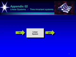
Appendix 02 Linear Systems - Time-invariant systems. Linear System. f(t). g(t). Linear System. A linear system is a system that has the following two properties:. Homogeneity :. Scaling :. The two properties together are referred to as superposition. Time-invariant System.

E N D
Appendix 02Linear Systems - Time-invariant systems Linear System f(t) g(t)
Linear System A linear system is a system that has the following two properties: Homogeneity: Scaling: The two properties together are referred to as superposition.
Time-invariant System A time-invariant system is a system that has the property that the the shape of the response (output) of this system does not depend on the time at which the input was applied. If the input f is delayed by some interval T, the output g will be delayed by the same amount.
Harmonic Input Function Linear time-invariant systems have a very interesting (and useful) response when the input is a harmonic. If the input to a linear time-invariant system is a harmonic of a certain frequency , then the output is also a harmonic of the same frequency that has been scaled and delayed:
Transfer Function H() The response of a shift-invariant linear system to a harmonic input is simply that input multiplied by a frequency-dependent complex number (the transferfunction H()). A harmonic input always produces a harmonic output at the same frequency in a shift-invariant linear system.
Transfer FunctionConvolution H() F() G() h(t) f(t) g(t)
Convolution h(t) f(t) g(t)
Impulse Response [2/4] h(t) f(t) g(t) H() F() G()
Some Useful Functions A B a/2 b
The Impulse Function [1/2] The impulse is the identity function under convolution
Discrete 1-Dim Convolution [4/5]Graph - Continuous / Discrete
Discrete Two-Dimensional Convolution [3/3] Kernel matrix Input image Output image Array of products x C Output pixel Summer Scaling factor
Linear System - Fourier Transform Impulse respons f(t) g(t) Input function h(t) H() Output function Spectrum of input function F() G() Spectrum of output function Transfer function