Download
1 / 21
210 likes | 287 Vues
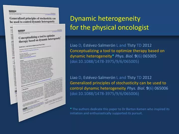
Dynamic heterogeneity for the physical oncologist. Liao D, Estévez-Salmerón L and Tlsty TD 2012 Conceptualizing a tool to optimize therapy based on dynamic heterogeneity * Phys. Biol. 9 (6) 065005 (doi:10.1088/1478-3975/9/6/065005 ) Liao D, Estévez-Salmerón L and Tlsty TD 2012

E N D
Dynamic heterogeneity for the physical oncologist Liao D, Estévez-Salmerón L and Tlsty TD2012 Conceptualizing a tool to optimize therapy based on dynamic heterogeneity*Phys. Biol.9(6) 065005 (doi:10.1088/1478-3975/9/6/065005) Liao D, Estévez-Salmerón L and Tlsty TD2012 Generalized principles of stochasticity can be used to control dynamic heterogeneityPhys. Biol.9(6)065006 (doi:10.1088/1478-3975/9/6/065006) *The authors dedicate this paper to Dr Barton Kamen who inspired its initiation and enthusiastically supported its pursuit.
Ø Dynamic heterogeneity for the physical oncologist Ø Seeming randomness Outcome vs. frequency Interconversion 0 1 2 3
Timings of biochemical reactions can seem to display randomness
Timings of biochemical reactions can seem to display randomness 0 1 2 3 4
Timings of biochemical reactions can seem to display randomness 0 1 2 3 4
Timings of biochemical reactions can seem to display randomness Messy variety of durations between events Unpredictability: Varied outcomes no protein 0 1 2 3 4
Ø Dynamic heterogeneity for the physical oncologist Ø Seeming randomness Outcome vs. frequency Interconversion 0 1 2 3
Phenotypes can be stochastic and interconvert no product Relatively resistant Protein in cell A Relatively sensitive Protein in cell B 0 1 2 3 4 5 6 7 8 9 10
Use Markov models to approximate phenotypic transitions ti ti + Dt Protein in cell 0 1 2 3 4 5 6 7 8 9 10
Use Markov models to approximate phenotypic transitions ti rR mS Ø cR cS Ø mR rS f ti + Dt Protein in cell 0 1 2 3 4 5 6 7 8 9 10
Ø Dynamic heterogeneity for the physical oncologist Ø Seeming randomness Outcome vs. frequency Interconversion 0 1 2 3
Metronomogram Ø Given: Ø Cannot directly kill “R” Illustrate: When can deplete S + R Cell kill Cell kill (t = 0) N(0+) Dt N(Dt-) Cell kill (t = Dt) N(Dt+) TCD Cell kill
Metronomogram Ø Killed Given: Ø Cannot directly kill “R” Illustrate: When can deplete S + R Cell kill Cell kill (t = 0) N(0+) Dt N(Dt-) Cell kill (t = Dt) N(Dt+) TCD Cell kill
Metronomogram Ø Killed Given: Ø Cannot directly kill “R” Illustrate: When can deplete S + R Cell kill Cell kill (t = 0) N(0+) Dt N(Dt-) Cell kill (t = Dt) N(Dt+) TCD Expansion Cell kill
Metronomogram Ø Killed Given: Ø 1.0 Cannot directly kill “R” Illustrate: When can deplete S + R 0.8 > Cell kill 0.6 Sensitized fraction 0.4 Cell kill (t = 0) N(0+) 0.2 Dt N(Dt-) Cell kill (t = Dt) 0 0.2 0.4 0.6 0.8 1.0 N(Dt+) Population expansion fraction TCD Expansion Cell kill
Metronomogram Ø Given: Ø 1.0 Cannot directly kill “R” Illustrate: When can deplete S + R 0.8 Cell kill 0.6 Sensitized fraction 0.4 Cell kill (t = 0) N(0+) 0.2 Dt N(Dt-) Cell kill (t = Dt) 0 0.2 0.4 0.6 0.8 1.0 N(Dt+) Population expansion fraction TCD Cell kill
Metronomogram Ø Given: Ø 1.0 Cannot directly kill “R” Illustrate: When can deplete S + R 0.8 S and R 0.6 R only Sensitized fraction 0.4 S and R R only N(0+) 0.2 Dt S and R N(Dt-) 0 0.2 0.4 0.6 0.8 1.0 R only N(Dt+) Population expansion fraction
Metronomogram Ø Given: Ø 1.0 Cannot directly kill “R” Illustrate: When can deplete S + R 0.8 S and R 0.6 R only Sensitized fraction 0.4 S and R R only N(0+) 0.2 Dt S and R N(Dt-) 0 0.2 0.4 0.6 0.8 1.0 R only N(Dt+) Population expansion fraction
Metronomogram Ø Given: Ø 1.0 Cannot directly kill “R” Illustrate: When can deplete S + R 0.8 Cell kill 0.6 Expansion and interconversion Sensitized fraction 0.4 Cell kill (t = 0) N(0+) 0.2 Dt N(Dt-) Cell kill (t = Dt) 0 0.2 0.4 0.6 0.8 1.0 N(Dt+) Population expansion fraction TCD Cell kill
Ø Dynamic heterogeneity for the physical oncologist Ø Seeming randomness Outcome vs. frequency Interconversion 0 1 2 3
Dynamic heterogeneity for the physical oncologist Liao D, Estévez-Salmerón L and Tlsty TD2012 Conceptualizing a tool to optimize therapy based on dynamic heterogeneity*Phys. Biol.9(6) 065005 (doi:10.1088/1478-3975/9/6/065005) Liao D, Estévez-Salmerón L and Tlsty TD2012 Generalized principles of stochasticity can be used to control dynamic heterogeneityPhys. Biol.9(6)065006 (doi:10.1088/1478-3975/9/6/065006) *The authors dedicate this paper to Dr Barton Kamen who inspired its initiation and enthusiastically supported its pursuit.