Download
1 / 36
360 likes | 370 Vues
Chapter 5 Climate Models. 5.1 Constructing a Climate Model. 5.2 * Numerical representation of atmospheric and oceanic equations. 5.3 Parameterization of small scale processes. 5.4 Climate simulations and climate drift. 5.5 ** The hierarchy of climate models.

E N D
Chapter 5Climate Models 5.1 Constructing a Climate Model 5.2*Numerical representation of atmospheric and oceanic equations 5.3 Parameterization of small scale processes 5.4 Climate simulations and climate drift 5.5**The hierarchy of climate models 5.6 Evaluation of climate model simulations for present day climate *Skip except mention of Fig. 5.9, **Skim Neelin, 2011. Climate Change and Climate Modeling, Cambridge UP
5.1 Constructing a Climate Model Typical atmospheric GCM grid • For each grid cell, single value of each variable (temp., vel.,…) • ÞFinite number of equations • Vertical coordinate follows topography, grid spacing varies • Transports (fluxes) of mass, energy, moisture into grid cell ÞBudget involving immediate neighbors (in balance of forces, PGF involves neighbors) • Effects passed from neighbor to neighbor until global • Budget gives change of temperature, velocity, etc., one time step (e.g. 15 min) later • 100yr=4million 15min steps Figure 5.1 Neelin, 2011. Climate Change and Climate Modeling, Cambridge UP
5.1.b Treatment of sub-grid scale processes Vertical column showing parameterized physics so smallscale processes within a single column in a GCM Figure 5.2 Neelin, 2011. Climate Change and Climate Modeling, Cambridge UP
5.1.c Resolution and computational cost Topography of western North America at 0.3° and 3.0° resolutions Figure 5.3 Neelin, 2011. Climate Change and Climate Modeling, Cambridge UP
Supplemental: Topography of North America at 0.5° and 5.0° resolutions Neelin, 2011. Climate Change and Climate Modeling, Cambridge UP
Computational time = (computer time per operation) ´(operations per equation)´(No. equations per grid-box) ´(number of grid boxes)´(number of time steps per simulation) Increasing resolution: # grid boxes increases & time step decreases Half horizontal grid size Þ half time step (why? See below) Þ twice as many time steps to simulate same number of years Doubling resolution in x, y & z Þ 2´2´2´(# grid cells) ´2´(# of time steps) Þ cost increases by factor of 24 =16 In Fig. 5.3, 5 to 0.5 degrees Þ factor of 10 in each horizontal direction. So even if kept vertical grid same,10´10´(# grid cells)´10´(# of t steps)= 103 Suppose also double vertical res. Þ 2000 times the computational time i.e. costs same to run low-res. model for 40 years as high res. for 1 week To model clouds, say 50m res. Þ 10000 times res. in horizontal, if same in vertical and time Þ 1016 times the computational time … and will still have to parameterize raindrop, ice crystal coalescence etc. 5.1.c Resolution and computational cost Neelin, 2011. Climate Change and Climate Modeling, Cambridge UP
Why time step must decrease when grid size decreases: Time step must be small enough to accurately capture time evolution and for smaller grid size, smaller time scales enter. A key time scale: time it takes wind or wave speed to cross a grid box. e.g., if fastest wind 50 m/s, crosses 200 km grid box in ~ 1 hour If time step longer, more than 1 grid box will be crossed: can yield amplifying small scale noise until model “blows up” (for accuracy, time step should be significantly shorter) [See Fig. 5.9 for an example of this] Examples of model resolutions in IPCC (2007) report: coarse 5´4°; typical ~2´2°; high 1° to 1.5° in lat. and longitude Computational costs cont’d Neelin, 2011. Climate Change and Climate Modeling, Cambridge UP
5.1.d An ocean model and ocean-atmosphere coupling Longitude-height cross-section through an ocean model grid Figure 5.4 Neelin, 2011. Climate Change and Climate Modeling, Cambridge UP
Atmosphere-ocean coupling in a GCMvia energy fluxes and wind stress Figure 5.5 Neelin, 2011. Climate Change and Climate Modeling, Cambridge UP
5.1.d Land surface, snow, ice, and vegetation Land surface types Figure 5.6 Neelin, 2011. Climate Change and Climate Modeling, Cambridge UP
Summary of equations for atmosphere and ocean models Table 5.1 Neelin, 2011. Climate Change and Climate Modeling, Cambridge UP
5.2 Numerical representation of atmos. and oceanic eqns. Finite differencing of a pressure field 5.2.a Finite difference versus spectral models [Skip] Figure 5.7 Neelin, 2011. Climate Change and Climate Modeling, Cambridge UP
Spectral representation of a pressure field [Skip] Figure 5.8 Neelin, 2011. Climate Change and Climate Modeling, Cambridge UP
5.2.b Time-stepping and numerical stability Simple time stepping scheme [Skim] Figure 5.9 Time step Dt must be small compared to physical time scales, here decay time t, or extrapolating slope can give erroneous growth ¶T′/ ¶t=−T′/tÞ(T′n+1-T′n)/Dt = −T′n/t For advection, Dt must be small rel. to timescale to cross grid box u/Dx Neelin, 2011. Climate Change and Climate Modeling, Cambridge UP
5.2.c Staggered grids "C" - Staggered grid [Skip] Figure 5.10 Neelin, 2011. Climate Change and Climate Modeling, Cambridge UP
5.3 Parameterization of small scale processes Vertical mixing and fluxes of moisture 5.3a Mixing and surface fluxes Figure 5.11 • Net flux across face of grid box due to mixing by smaller scale motions parameterized as proportional to difference in q at levels k, k-1 • Evaporation flux of surface depends on difference between lowest level q and saturation value at surface Neelin, 2011. Climate Change and Climate Modeling, Cambridge UP
5.3b Dry convection Change in environmental lapse rate [Skip] Figure 5.12 Neelin, 2011. Climate Change and Climate Modeling, Cambridge UP
5.3c Moist convection Parcel stability [Skip] Figure 5.13 Neelin, 2011. Climate Change and Climate Modeling, Cambridge UP
5.3d Land surface processes and soil moisture Land surface model: soil moisture and evapotranspiration Evapotranspiration Precipitation Aerodynamic resistance Canopy Interception Leaf area index Canopy (stomatal) resistance Runoff Soil moisture Soil capacity Figure 5.14 Neelin, 2011. Climate Change and Climate Modeling, Cambridge UP
5.3e Sea ice and snow Sea ice model processes Figure 5.15 Neelin, 2011. Climate Change and Climate Modeling, Cambridge UP
5.4 The hierarchy of climate models [Skip] Table 5.2 Neelin, 2011. Climate Change and Climate Modeling, Cambridge UP
5.5 Climate simulations and climate drift Climate drift Figure 5.16 Examples of model integrations (or runs, simulations or experiments), starting from idealized or observed initial conditions. Spin-up to equilibrated model climatology is required (centuries for deep ocean). Model climate differs slightly from observed (model error aka climate drift); climate change experiments relative to model climatology. Neelin, 2011. Climate Change and Climate Modeling, Cambridge UP
5.6 Evaluation of climate model simulations for present day climate Atm. component of NCAR_CCSM3 forced by observed SST (AMIP)Precipitation Climatology 1979-2000with observed (CMAP) 4mm/day contour December-February 5.6a Atmos. model clim. from specified SST June - August AMIP=Atm. Model Intercomparison Project CMAP=CPC Merged Analysis of Precip. CPC=NOAA Climate Prediction Center CCSM=Community Climate System Model Figure 5.17 Neelin, 2011. Climate Change and Climate Modeling, Cambridge UP
Observed (CMAP) Precipitation Climatology 1979-2000 December-February Recall from Fig. 2.13 June - August Neelin, 2011. Climate Change and Climate Modeling, Cambridge UP
5.6b Climate model simulation of climatology 4 mm/day Precipitation climatology contour Observed (CMAP) and coupled/uncoupled model December-February NCAR_CCSM3 Coupled simulation climatology (20th century run, 1979-2000)& Atmospheric component forced by obs. SST (AMIP) June - August Figure 5.18 Neelin, 2011. Climate Change and Climate Modeling, Cambridge UP
HadCM3 simulation precipitation climatology (20th century run, 1961-1990) January July Figure 5.19 Neelin, 2011. Climate Change and Climate Modeling, Cambridge UP
Observed (CMAP) Precipitation Climatology 1979-2000 January July Recall Figure 2.13 Neelin, 2011. Climate Change and Climate Modeling, Cambridge UP
Observed (CMAP) and 5 coupled models 4 mm/dayprecip. contour December-February Coupled simulation precipitation climatology (20th century run, 1979-2000) June - August Figure 5.20 Neelin, 2011. Climate Change and Climate Modeling, Cambridge UP
Observed (CMAP) and 7 other coupled models 4 mm/dayprecip. contour December-February Coupled simulation precipitation climatology (20th century run, 1979-2000) June - August Supplemental Figure Neelin, 2011. Climate Change and Climate Modeling, Cambridge UP
December-February NCAR_CCSM3 coupled simulationSST climatology (20th century run, 1979-2000) June - August Figure 5.21 Neelin, 2011. Climate Change and Climate Modeling, Cambridge UP
January Observed SST climatologyReynolds data set (1982-2000) July Recall Figure 2.16 Neelin, 2011. Climate Change and Climate Modeling, Cambridge UP
January HadCM3 coupled simulation near surface air temperature (20th century run,1961-1990) July Figure 5.22 Neelin, 2011. Climate Change and Climate Modeling, Cambridge UP
Figure 5.23 Regions of sea ice concentrations > 15% for Mar. & Sept. • March (light shading/blue contour) • September (dark shading/pink contour) • Contours repeat observed for comparison on 2 model simulations Neelin, 2011. Climate Change and Climate Modeling, Cambridge UP
5.6c Simulation of ENSO response Precipitation anomaly (mm/day) for Dec.-Feb. for the average of 5 El Nino events minus the average of 5 La Nina events CMAP Obs AMIP CCSM3 AMIP MRI Figure 5.24 Neelin, 2011. Climate Change and Climate Modeling, Cambridge UP
Precipitation anomaly (mm/day) for Dec.-Feb. for the average of 5 El Nino events minus the average of 5 La Nina events CMAP Obs Shaded where statistically significant at 95% level. AMIP CCSM3 AMIP MRI Figure 5.24 alternate Neelin, 2011. Climate Change and Climate Modeling, Cambridge UP
Upper tropospheric (200mb) geopotential height anomaly (mm/day) for Dec.-Feb. for the avg of 5 El Nino events minus the avg of 5 La Nina events NCEP reanalysis (observational product) Figure 5.25 AMIP CCSM3 AMIP MRI NCEP=National Centers for Environmental Prediction; Reanalysis has observations interpolated via a weather forecast model AMIP=Atm. Model Intercomparison Project CCSM=Community Climate System Model Neelin, 2011. Climate Change and Climate Modeling, Cambridge UP