Download
1 / 43
440 likes | 579 Vues
Some Uses of Channel Bed Sediment Concentration Data. Determine the spatial distribution of trace metals Identify point and non-point sources of pollution Assessment of the rates and patterns of contaminant dispersal

E N D
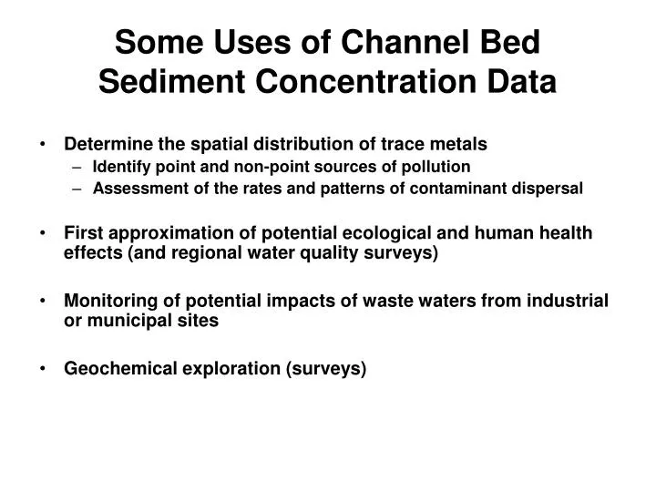
Some Uses of Channel Bed Sediment Concentration Data • Determine the spatial distribution of trace metals • Identify point and non-point sources of pollution • Assessment of the rates and patterns of contaminant dispersal • First approximation of potential ecological and human health effects (and regional water quality surveys) • Monitoring of potential impacts of waste waters from industrial or municipal sites • Geochemical exploration (surveys)
Downstream Trends in Channel Bed From Salomons & Forstner, 1984 • Where point sources are present the concentrations generally decline from the point of input.
Concentrations of Cu and Ni in the <63 um fraction of channel bed sediments from the Po River, Italy. Samples were collected in the summer (grey bars) and winter (black bars). Acronyms along x-axis represent successive downstream sampling sites. Note minimal variations in concentration between seasons. Viganò, L., and 14 others, 2003. Quality assessment of bed sediments of the Po River (Italy). Water Research, 37:501-518. (from 2 of 8 graphs from figure 3, page 507)
Downstream Trends in Channel Bed From Salomons & Forstner, 1984 • Where point sources are present the concentrations generally decline from the point of input.
Characteristics of channel deposits (adapted from Knighton 1998; Church and Jones 1982; Hoey 1992)
Figure from Huggett, J.R., 2003. Fundamental of Geomorphology, Routledge Fundamentals in Physical Geography, Routledge, London, fig. 7.7, p. 185.
Straight Channel Meandering Channel (A) Longitudinal Profile (B) (C) Riffle Mean Water Surface Slope Riffle Elevation Pool Pool Riffle Distance Downstream
Super Elevated Water Surface Point Bar Secondary Flow Directions From Markham, A.J. and Thorne, C.R., 1992. Geomorphology of gravel-bed river bends. In: P. Billi, R.D. Hey, C.R. Thorne, and P. Tacconi, (eds.), Dynamics of Gravel-bed Rivers, pp. 433-456, New York, Jonh Wiley and Sons, Ldt., figure 22.2, p. 436.
From Thompson, A., 1986. Secondary Flows and the Pool-Riffle, Earth Surface Processes and Landforms, 11:631-641., Figure 4, p. 636.
Reading, H.G., 1978. Sedimentary Environments and Facies, Blackwell Publications, New York, Fig. 3.26, page 34. Company may have been purchased by Elsevier?
Figure 20. Laremie River, Wyoming (photo by J.R. Balsley); obtained from USGS Photo Library
Knighton, D., 1998. Fluvial Form and Processes: A New Perspective, Arnold, London. Fig. 5.23, p. 233.
Grain-Size & Compositional Variations • Ladd et al. 1998 • Examined trace metal concentrations in 7 morphological units in Soda Butte Creek, Montana • (lateral scour pools, eddy drop zones, glides, low gradient riffles, high gradient riffles, attached bars, and detached bars) • Highest concentrations in eddy drop zones and attached lateral bars with largest amount of fine sediment
Density-Dependent Variations • Slingerland and Smith (1986) define a placer as “a deposit of residual or detrital mineral grains in which a valuable mineral has been concentrated by a mechanical agent,” • A contaminant placer is defined here as a concentration of metal enriched particles by the hydraulic action of the river. Where they occur, trace metal concentrations will be locally elevated in comparison to other areas(Miller & Orbock Miller, 2007)
Guilbert, J.M. and Park, C.F., Jr., 1986. The Geology of Ore Deposits. New York, W.H. Freemand and Company, figures 16-1, p. 746 and 16-4b p.749.
Bateman, A.M., 1950. Economic mineral deposits, 2nd edition. New York, Wiley and Sons.
Reno Fallon Lahontan Reservoir Virginia i l M e City x C i a 95 Fort S n y o Table n Churchill 15 Six Mile Mtn. 11 18 Canyon Fan 14 13 16 17 9 10 Mineral 7C 12 Canyon 7D Gaging Station Gold Canyon 7B 7 6 Dayton 5 4 Pyramid 3 Lake 2B Canyon (Brunswick) Carson 2 City T Carson 1B r u Playa c k e Stillwater e 1 R Wildlife . . R Refuge n o s r a C 395 0 . R Gaging Lahontan e e k c station Carson Reservoir u r Lake T . . R Lake n o Carson River s Tahoe r a C Watershed Boundary Carson City k r o F E a t s s t e 0 1 2 3 4 5 W Miles F F o 0 1 2 3 4 Km o r r k k SIERRA NEVADA Nevada California
Variations Dependent on Time and Frequency of Inundation • Examples • Queens Creek, Arizona • Rio Pilcomayo, Bolivia
Graf, W.L., Clark, S.L., Kammerer, M.T., Lehman, T., Randall, K., Tempe, R., and Schroeder, A., 1991. Geomorphology of heavy metals in the sediments of Queen Creek, Arizona, USA. Catena, 18:567-582, figures 2, p. 572 and 6, p. 578.
Study Area
Floatation Process “Modern Mine” Pb & Zn Concentrate Ball Mill
Sampling Site RP-1 ~1.5 miles from Mills Floatation Mill, Potosi Effluent You want me to live where? 20 miles from Mills
~60 miles from Mills 20 miles from Mills
High-Water Channel Deposits Low-Water Channel Deposits Rio Pilcomayo, southern Bolvia near Uyuni. Photo taken in July during the dry season.
Implications to Sampling • Local variations – referred to as small scale or field variance (Birch et al. 2001) • Can be on the order of 10 to 25 % relative standard deviation and may be significantly greater than analytical variation (error) • May hinder ability to decipher differences in contaminant levels between sample sites • Reconnaissance level surveys and sample stratification by morphological units ? • Sampling of specific units only? • Composite sampling to minimize within unit variations
Changes in Sediment Composition Can: • Influence the spatial and temporal concentration patterns observed in aquatic systems • Hinder the determination of localized inputs of trace metals from either natural sources (e.g., ore bodies) or anthropogenic sources (e.g., mining operations or industrial complexes). • Changes in grain-size have a particularly significant influence on metal concentrations.
Types of Mathematical Manipulations Commonly Applied to Bulk Metal DataAfter Horowitz, 1991 • Corrections for Grain-size differences • Normalization to a single grain-size range • Carbonate content corrections • Recalculation of concentration data on a carbonate-free basis • Normalization to a conservative elemental • Use of multiple Normalizations
Methods of Handling the Grain Size Effect • Analysis of a specific grain-size fraction which is considered to be the chemical active phase • Does not provide for an understanding of the actual concentrations that exist in the bulk sample • Inhibits the calculation of total trace metal transport rates • Normalize the metal concentration data obtained for the bulk (< 2mm or sand) sized fraction using some form of mathematical equation and grain size data obtained from a separate sample • Provides actual concentration found in bulk sample • Poorly documents the concentrations that would actually be measured in the finer-grain size fractions
Designation of Chemical Active Sediment Phase • Numerous size fractions have been used as the chemical active phase including <2 µm, <16 µm, <20 µm, <63 µm, <70 µm, <155 µm, <200 µm (Horowitz, 1991) • Argument for using < 63 µm fraction • It can be extracted from the bulk sample via sieving, a process which does not alter trace metal chemistry • It is the particle size most commonly carried in suspension by rivers and streams and may therefore be the most readily distributed through the aquatic environment
Grain Size Normalization Normalized Concentration = (DF *Bulk Metal Concentration) Where, DF = Dilution Factor = 100/(100 - % of sediment > size range of Interest)
Concentration vs. Quantity of Fine Sediment • Sizes Frequently Used • 2 μm • 16 μm • 62.5 μm • 63 μm • 70 μm • 125 μm • 200 μm Data from deGroot et al., 1982
Differences between Measured and Normalized Values • Selected chemical active phase (grain size fraction) may not contain all of the trace metals • Differences in concentration are not solely due to grain size variations • Data contain analytical errors associated with grain size or geochemical analyses
Fractional Contributions of Selected Metals in Suspended Sediments (modified from Horowitz et al., 1990)
Normalized Concentration (DF *Bulk Metal Concentration) = Carbonate Correction • Assumes: Carbonate does not contain substantial quantities of trace metals and, thus, acts as a diluent. May not be true of Cd and Pb. • Generally applied to streams in calcareous terrains, particularly those in areas with karst. Where, DF = Dilution Factor = 100/(100 - % of carbonate in sample)
Conservative Element Corrections • Assumes that some elements have had a uniform flux from crustal rocks. Thus, normalization to these elements provides a measure (or level) of dilution that has occurred. • Elements most commonly used are Al, Ti, and to a lesser extent, Cs and Li. • Normalized value = (Concentration of Trace Metal) (Concentration of conservative element) Note: this generates a ratio, not a concentration as did the previous procedures