Download
1 / 1
10 likes | 88 Vues
Figure 2. Results after 100kyr in the standard experiment. The three panels show ice thickness (upper panel in m), downstream velocity (middle panel in m yr -1 ) and the ratio of basal traction to gravitational driving stress (lower panel).

E N D
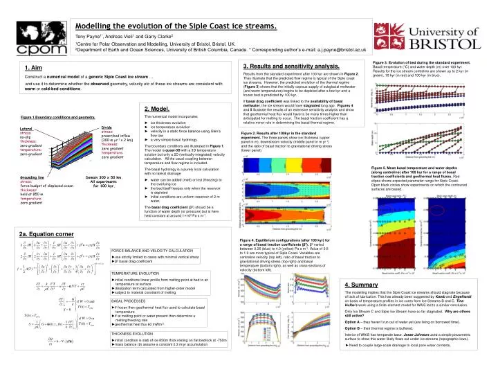
Figure 2. Results after 100kyr in the standard experiment. The three panels show ice thickness (upper panel in m), downstream velocity (middle panel in m yr-1) and the ratio of basal traction to gravitational driving stress (lower panel). Figure 3. Evolution of bed during the standard experiment. Basal temperature (°C) and water depth (m) over 100 kyr. Results for the ice stream centreline are shown up to 2 kyr (in green), 10 kyr (in red) and 100 kyr (in blue). Figure 1 Boundary conditions and geometry. Divide stress: prescribed inflow (300 m yr-1 x 2 km) thickness: zero gradient temperature: zero gradient Lateral stress: no-slip thickness: zero gradient temperature: zero gradient Grounding line stress: force budget of displaced ocean thickness: held at 850 m temperature: zero gradient Domain 300 x 50 km. All experiments for 100 kyr. Figure 5. Mean basal temperature and water depths (along centreline) after 100 kyr for a range of basal traction coefficients and geothermal heat fluxes. Red elipse shows expected parameter range for Siple Coast. Open black circles show experiments on which the contoured surfaces are based. 2a. Equation corner FORCE BALANCE AND VELOCITY CALCULATION ►use strictly limited to cases with minimal vertical shear ►β2 basal drag coefficient TEMPERATURE EVOLUTION ►initial conditions linear profile from melting point at bed to air temperature at surface ►dissipation term calculated from higher-order model ►subject to material constraint of melting Figure 4. Equilibrium configurations (after 100 kyr) for a range of basal traction coefficients (β2). β2 varied between 0.25 (blue) to 4.0 (yellow) Pa s m-1. Value of 0.5 to 1.0 are more typical of Siple Coast. Variables are centreline velocity (top left), ratio of basal traction to gravitational driving stress (top right) and basal temperature (bottom right), as well as cross-sections of velocity (bottom left). BASAL PROCESSES ►if frozen then geothermal heat flux used to calculate basal temperature ►if at melting point or water present then determine a melting/freezing rate ►geothermal heat flux 60 mWm-2 THICKNESS EVOLUTION ►initial condition is slab of ice 850m thick resting on flat bedrock at -750m ►mass balance (b) assume a constant 0.3 m/yr accumulation 3. Results and sensitivity analysis.Results from the standard experiment after 100 kyr are shown in Figure 2. They illustrate that the predicted flow regime is typical of the Siple coast ice streams. However, the predicted evolution of the thermal regime (Figure 3) shows that the initially copious supply of subglacial meltwater (and warm temperatures) begins to be depleted after a few kyr and a frozen bed is predicted by 100 kyr.If basal drag coefficient was linked to the availability of basal meltwater, the ice stream would have stagnated long ago. Figures 4 and 5 illustrate the results of an extensive sensitivity analysis and show that geothermal heat flux would have to be many times higher than anticipated for melting to occur. The basal traction coefficient has a relative minor role in determining the basal thermal regime. Modelling the evolution of the Siple Coast ice streams.Tony Payne1*, Andreas Vieli1 and Garry Clarke21Centre for Polar Observation and Modelling, University of Bristol, Bristol, UK.2Department of Earth and Ocean Sciences, University of British Columbia, Canada. * Corresponding author’s e-mail: a.j.payne@bristol.ac.uk 1. Aim Construct a numerical model of a generic Siple Coast ice stream …and use it to determine whether the observed geometry, velocity etc of these ice streams are consistent with warm or cold-bed conditions. 2. Model.The numerical model incorporates► ice thickness evolution► ice temperature evolution► velocity in a static force balance using Glen’s flow law► a very simple basal hydrology.The boundary conditions are illustrated in Figure 1. The model isquasi-3D with a 3D temperature solution but only a 2D (vertically-integrated) velocity calculation. All the usual coupling between temperature and flow regime is included.The basal hydrology is a purely local calculation with no lateral drainage ► water can be added (melt) or lost (freezing) to the overlying ice► the bed itself freezes only when the reservoir is depleted► initial conditions are uniform reservoir of 2 m water.The basal drag coefficient (β2) should be a function of water depth (or pressure) but is here held constant at around 1×10⁹ Pa s m-1. 4. SummaryThe modelling implies that the Siple Coast ice streams should stagnate because of lack of lubrication. This has already been suggested by Kamb and Engelhardt on basis of temperature profiles in ice cores from Ice Streams B and C. Tina Hulbe’s work using a finite-element model for WAIS led to a similar conclusion.Only Ice Stream C and Siple Ice Stream have so far stagnated. Why are others still active?Option A – they haven’t run out of water yet (are living on borrowed time).Option B – their thermal regime is buffered. Interior of WAIS has temperate base. Jesse Johnson used a simple piezometric surface to show this water likely flows out under ice streams (topographic lows).►Need to couple large-scale drainage to local pore water contents.