Download
1 / 39
390 likes | 483 Vues
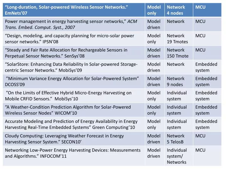
Networking Low-Power Energy Harvesting Devices: Measurements and Algorithm. Gorlatova M., Wallwater A., Zussman G. INFOCOM 2011. Outline . Introduction Model Measurement Energy profile Algorithm for predictable profile and stochastic profile Result . Introduction.

E N D
Networking Low-Power Energy Harvesting Devices: Measurements and Algorithm Gorlatova M., Wallwater A., Zussman G. INFOCOM 2011
Outline • Introduction • Model • Measurement • Energy profile • Algorithm for predictable profile and stochastic profile • Result
Introduction • Achieve time-fair resource allocation since energy varies among different time • Other research focus on fairness • Data generation rate (SenSys08) • among nodes (JSAC06) • Proposed energy allocation algorithms across the different time slot to optimize • energy spending rate for single node • energy communication rate for a link • Indoor irradiance measurements study.
Dimensions of algorithm design • Environmental energy model • Energy storage type • Ratio of energy storage capacity to energy harvested • Time granularity • nodes characterize received energy • Make decision from sec ~days • Problem /Network size • energy harvesting affects nodes’ decisions • Link decisions, routing, rate adaptation
Environmental energy model • Predictable profiles • Ideal • Accurate for the future • Partially predictable • Stochastic • Model-free
Energy storage type • Rechargeable battery • Ideal linear model • Changes of stored energy vs harvested power • Capacitor • Non-linear model • Power harvested depend both on the energy provided and on the amount of energy stored
Contributions • Indoor : partially-predictable energy model • Time granularity : day, improving prediction • Fair allocation of resources along the time • Energy spending rate for a node • Data rate for a link • Predictable energy profiles • Lexicographic maximization • Utility maximization • Stochastic model • Markov Decision Process
Model • K slots time i = {0,1,…K-1} • D=AηH • Q(i)=q(D(i),B(i)) for capacitor
Objective • Optimization energy spending rate s(i) for single node • Optimization energy communication rate ru(i), rv(i) for a link • Utility maximization frame work to find • spending rate s(i) • communication rate ru(i), rv(i) • α-fair function U(s(i)) = s(i)1-α/(1-α), for α>0, α≠1 log(s(i)), for α=1 • Consider predictable profile energy model
Dynamic programming-based algorithm • h(i,B(i))=max[ U(s(i)) + h(i+1,min(B(i)+Q(i)-s(i),C))] • Determine vector {s(0),…s(K-1)} maximizes h(0,B0) • Running time O(K[C/△]2)
For linear storage q(D(i),B(i)) = D(i) • Progressive Filling algorithm • Running time O(K[K+QT/△]),QT= ΣQ(i)+(B0-BK) • If linear storage is large, s(i) = QT/K
Measurement • Long-term measurement of indoor irradiance • Office buildings at Columbia Uni. since 2009/6 • TAOS TSL230rd photometric sensors • LabJack U3 DAQ
Hd: mean of the daily irradiation • σ : standard deviation • r : bit rate, throughout a day when exposed Hd • r = A(10cm2) x η(1%) x Hd /(3600x24)/(10e-9) • EnHANTs costs 1nJ/bit
How to predict Hd? • Exponentially weighted moving-average (EWMA) • Error is relatively high • For L-1, avg. prediction error > 0.4Hd • L-2, avg. prediction error > 0.5Hd • Outdoor, avg. prediction error = 0.3Hd • Weather forecast [secon10] may be improved • For L-1, correlation coefficient of Hd and weather = 0.35 • For L-6, correlation coefficient =0.8
Work week pattern • For L-2, student office, on shelf far from window • Hd= 1.63 on weekdays, Hd=0.37 on weekend • 9.7hr/day lighting on weekday, <1hr on weekend • Avg. error prediction error 0.5Hd -> 0.26Hd if separate weekdays and weekends. • L-1 and L-5, correlation coefficient =0.58 • L-1 and L-5 facing same direction, correlation coefficient =0.71
Short term energy profiles • HT, T= 0.5 hr • L-3, daylight-dependent variations • L-2, either 0 or 45uW/cm2 • partially predictable energy model
Mobile measurements • mobile device carried around indoor and outdoor locations • Indoor : 70uW/cm2 • Outdoor : 32mW/cm2 • Poorly predictable • Stochastic energy model
Extension of TFR algorithm • {ru(0),..ru(K-1)}, {rv(0,..rv(K-1)} maximize h(0,B0u,B0v) • Complexity : • For linear storage, LPF algo.,
Decoupled Rate Control algorithm • DRC algorithm • Determine su(i), sv(i) independently using PF algorithm • r(i) = min(su(i), sv(i))/(ctx + crx)
Stochastic Energy model • Energy harvested in a slot is and i.i.d (identical independent distribution)random variable D • [d1,..dM] with probability [p1,…pM] • Spending Policy Determination (SPD) problem • Given distribution D, determine s(i) • Markov Decision Process(MDP)
Apply dynamic programming, from i=K-1 for each {i,B(i)} • For each storage B(i), s(i) approached optimal • Running time
Link Spending Policy Determination Problem(LSPD) • Apply dynamic programming • For each {i, Bu(i), Bv(i)} • Maximization is over all {ru(i), rv(i)}, such that • ctxru(i) + crxrv(i) = su(i) ≤ Bu(i) • ctxrv(i) + crxru(i) =sv(i) ≤ Bv(i) • Complexity: O([Cu/△]2[Cv/]2MuMvK)
Numerical results • Energy profile L-3 input • s(i) are obtained by PF algorithmfor linear storage(left) • s(i) for TFU problem for nonlinear storage (right)
L-1, L-2 energy profile • Optimal communication rate {ru(i), rv(i)}
Optimal energy spending policies (SPD) • L-1 profile as random variable D • Optimal s(i) • Optimal communication rateru(i), rv(i)
Conclusion • First long-term indoor radiant energy measurements campaign that provides useful traces • Developed algorithms for predictable environment that uniquely determine the spending policies for linear and non-linear energy storage models • Developed algorithms for stochastic environments that can provide nodes with simple pre-computed decisions policies
Alpha ->0, globally optimize • Alpha ->1, proportional fairness • ->2, harmonic mean fairness • -> infinite , generalized max min allocation
Introduction • Perpetual energy harvesting wireless device • Solar, piezoelectric and thermal energy harvesting • Ultra-low-power wireless communication • Rechargeable sensor networks • Focus on devices that harvest environmental light energy • Energy-harvesting-aware algorithm and system • Lack of data and analysis of energy availability for indoor/outdoor environment • 16 months indoor light energy measurement • light measurement and resource allocation