Download
1 / 15
150 likes | 253 Vues
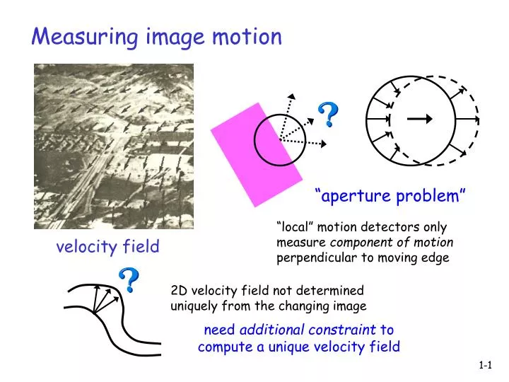
Measuring image motion. “aperture problem”. “local” motion detectors only measure component of motion perpendicular to moving edge. velocity field. 2D velocity field not determined uniquely from the changing image. need additional constraint to compute a unique velocity field.

E N D
Measuring image motion “aperture problem” “local” motion detectors only measure component of motion perpendicular to moving edge velocity field 2D velocity field not determined uniquely from the changing image need additional constraint to compute a unique velocity field
Assume pure translation or constant velocity Vy • Error in initial motion measurements • Velocities not constant locally • Image features with small range of orientations Vx In practice…
Measuring motion in one dimension I(x) Vx x • Vx = velocity in x direction • rightward movement: Vx > 0 • leftward movement: Vx < 0 speed: |Vx| • pixels/time step I/x + - + - I/t I/t I/x Vx = -
Measurement of motion components in 2-D (1) gradient of image intensity I = (I/x, I/y) (2) time derivative I/t (3) velocity along gradient: v movement in direction of gradient: v > 0 movement opposite direction of gradient: v < 0 +x +y true motion motion component I/t [(I/x)2 + (I/y)2]1/2 I/t |I| v = - = -
2-D velocities (Vx,Vy) consistent with v (Vx, Vy) (Vx, Vy) Vy v Vx All (Vx, Vy) such that the component of (Vx, Vy) in the direction of the gradient is v (ux, uy): unit vector in direction of gradient Use the dot product: (Vx, Vy) (ux, uy) = v Vxux + Vyuy = v
In practice… Previously… Vy Vxux + Vy uy = v New strategy: Find (Vx, Vy) that best fits all motion components together Vx Find (Vx, Vy) that minimizes: Σ(Vxux + Vy uy - v)2
Smoothness assumption: • Compute a velocity field that: • is consistent with local measurements of image motion (perpendicular components) • has the least amount of variation possible
Computing the smoothest velocity field (Vxi-1, Vyi-1) motion components: Vxiuxi + Vyi uyi= vi (Vxi, Vyi) (Vxi+1, Vyi+1) i-1 i i+1 change in velocity: (Vxi+1-Vxi, Vyi+1-Vyi) Find (Vxi, Vyi) that minimize: Σ(Vxiuxi + Vyiuyi - vi)2 + [(Vxi+1-Vxi)2 + (Vyi+1-Vyi)2]
Ambiguity of 3D recovery birds’ eye views We need additional constraint to recover 3D structure uniquely “rigidity constraint”
perspective projection Image projections orthographic projection Z Z image plane X X image plane (X, Y, Z) (X/Z, Y/Z) (X, Y, Z) (X, Y) only scaled depth requires translation of observer relative to scene only relative depth requires object rotation
Incremental Rigidity Scheme x depth: Z initially, Z=0 at all points (x1 y1 z1) (x3 y3 z3) y (x1' y1' ??) (x3' y3' ??) Find new 3D model that maximizes rigidity (x2 y2 z2) (x2' y2' ??) Compute new Z values that minimize change in 3D structure image
Bird’s eye view: Z lij depth Lij x image current model Find new Zi that minimize Σ (Lij – lij)2/Lij3 new image
Observer motion problem, revisited From image motion, compute: Observer translation (Tx Ty Tz) Observer rotation (Rx Ry Rz) Depth at every location Z(x,y) Observer undergoes both translation + rotation
Longuet-Higgins & Prazdny • Along a depth discontinuity, velocity differences depend only on observer translation • Velocity differences point to the focus of expansion