Download
1 / 27
270 likes | 396 Vues
P rogress of creating future wind speed forcing for VIC runs Xiaodong. Oct 1, 2013. 1. Project Background. Assessment of the Vulnerability of Permafrost Carbon to Climate Change: A Sensitivity Analysis among Models PI: Dave McGuire. Question:

E N D
Progress of creating future wind speed forcing for VIC runs Xiaodong Oct 1, 2013
1. Project Background Assessment of the Vulnerability of Permafrost Carbon to Climate Change: A Sensitivity Analysis among Models PI: Dave McGuire Question: How would the carbon components in high-latitude permafrost change under the future climate change?
1. Project Background 1. Simulate the historical and behavior of high-latitude permafrost area around the Arctic basin Work flow • Results(hydrology components, • carbon cycle components) • DetrendedForcings • (de_temp • de_co2 • de_temp.de_prec) • Control runs • 1960-2006 required)
1. Project Background 2. Investigate the sensitivity of carbon cycle components toward future climate change (prec, temp, [co2]) Work flow RCP4.5 and RCP8.5 scenarios, anomaly-correction strategy VIC forcing: Precipitation Air temperature Wind speed (combined) Variables provided: Precipitation scale factors SurfT anomalies Wind (u & v) anomalies Wind (combined) anomalies
2. Forcing Issues 1. Info about how to use future forcing anomalies (From Dave Lawrence) Wind (combined) anomalies To create future wind forcings anomaly = future proj. - historical reference m: month (loop over 1-12) y: year (loop over 2006-2299) • One value for each month • From 1996-2005 climatology run of CCSM4 historical simulation (case name: b40.20th.track1.1deg.008) t: timestep (in our case it is day) yobs: loop over 1996-2005
2. Forcing Issues 2. Negative future wind speed
2. Forcing Issues Components of this negative future wind speed
2. Forcing Issues 3. Progress • Info about 2 types of forcing • Dave’s forcing is from CCSM future runs (case name: b40.rcp4_5.1deg.001 and b40.crp4_5.2300.001 and b40.20th.track1.1deg.008) • Our VIC forcing is from NCEP-NCAR reanalysis (Kalnay et al. 1996) • Lowest level of model output (in geopontentialheight), so lowest layer is about 35m • 1985-2004 Jan. average wind speed is 4.99m/s (cell 5895, at W.Siberia) • Fixed at 10m height • 1996-2005 Jan. average wind speed is 3.09m/s (cell 5895)
2. Forcing Issues 3. Progress Scaling the wind speed down to 10m • Surface roughness and displacement data is obtained from dataset for Stehekin River basin (same as Ted’s setting in the West Siberia run) Zd is displacement height(in m) Z0 is roughness (in m) Averaged ratio for whole domain is: 2.3452 (excludes water bodies and bare soil) 3.2804 (take water bodies and bare soil as max. roughness and displacement veg type on land)
2. Forcing Issues 3. Progress Scaling the wind speed down to 10m • Surface roughness and displacement data is obtained from dataset for Stehekin River basin (same as Ted’s setting in the West Siberia run) Zd is displacement height(in m) Z0 is roughness (in m) Averaged ratio for whole domain is: 2.3452 (excludes water bodies and bare soil) 3.2804 (take water bodies and bare soil as max. roughness and displacement veg type on land)
2. Forcing Issues 3. Progress Scaling the wind speed down to 10m For each cell: Total roughness and displacement is calculated based on the area fraction of each vegetation type. The total sum is then rescaled by total fraction. Ratio is calculated separately for each cell. For choice 1, total fraction=1-(wetfrac*water_frac)-(dryfrac*baresoil_frac); For choice 2, total fraction=1 Zd is displacement height(in m) Z0 is roughness (in m) Averaged ratio for whole domain is: 2.3452 (excludes water bodies and bare soil) 3.2804 (take water bodies and bare soil as max. roughness and displacement veg type on land)
2. Forcing Issues 3. Progress For this grid cell, the future wind speed looks fine. But for some cells there are still occasional negative wind speed.
2. Forcing Issues 3. Progress Further: Set min_wnd = 0.1m/s to complete avoid non-positive wind speed 0.1m/s is taken from VIC global parameter file For Dennis: Do you approve this further limiting?
Progress of methane (CH4) observation project Xiaodong Oct 1, 2013
1. Project Background Tower Assimilation of CH4 observation in West Siberia • Target: • Simulate the atmos [CH4] at towers in West • Siberia wetland area. • Working with Dr. ShamilMaksyutov at NIES
2. Progress 1. Feedback from last meeting Find out if there is any relationship between seasonal maximum [CH4] and ground water table depth and soil temperature For 3 of 4 stations, there is relation between them, but for minimum [CH4]. For 3 of 4 stations, there is relation between monthly avg [CH4] and monthly zwt, Tsurf, NPP , and wind stats. IGR station (see map below) is far away from main wetland area, so the relationship here is a little different. I excluded this station from my regressions below.
2. Progress 2. Station info
2. Progress 3. Relation for seasonal averaged [CH4] For JJA (summer high emission period): ZWT is always negative, same for the following regression. Issues: Limited data points
2. Progress 4. Relation for seasonal minimum [CH4] For JJA (summer high emission period): Issues: Limited data points Solution: Try monthly analysis
2. Progress 5. Relation for summer monthly average [CH4] 11 data points from summer months (June, July, August). Not JJA average. Use ZWT, Tsurf, NPP stats for regression
2. Progress 5. Relation for summer monthly average [CH4] • Possible application: • Available fro VIC :1948-2006 historical zwt, Tsurf and NPP simulation results • Use: Regression relationship • Produce: 1948-2006 historical [CH4] concentration. See if the trend is correct.
2. Progress 6. Relation for summer monthly average [CH4] DEM shows increasing trend (0.3586), as expected NOY shows decreasing trend (-0.2326), unexpected Possible Solution: Involve wind speed ?
2. Progress 5. Relation for all the available monthly average [CH4] 39 data points. Use ZWT, Tsurf, NPP and wnd_speed stats for regression
2. Progress 5. Relation for all the available monthly average [CH4] There is increasing trend (0.0006ppm/month) in this reconstructed series. Reconstruction of historical atmos [CH4] at DEM station
2. Progress 5. Relation for all the available monthly average [CH4] Reconstruction of historical atmos [CH4] at NOY station
2. Progress 5. Relation for all the available monthly average [CH4] Reconstruction of historical atmos [CH4] at KRS station
2. Progress 6. Conclusion • At stations DEM, NOY and KRS, atmosphere [CH4] observation at the lowest level (differ for each station) shows significant relationship (sig.F=0.000127<0.05) with CH4 emission rate and 10m wind speed. • CH4 emission rate is controlled by ground water table depth (zwt), surface soil temperature (Tsurf) and NPP. • Atmos [CH4] can be approximated by zwt, Tsurf, NPP and wnd statistics. • This approximation might be used to reconstruct the historicslatmosphere [CH4] at these 3 stations. • The reconstructed atmos [CH4] shows an increasing trend at all 3 stations. My current question is: The trend is correct, but what about the values (+0.0004ppb/month)?