Download
1 / 13
130 likes | 134 Vues
This exercise materials prepared by Joseph K. Berry explores the concept of forest availability and accessibility in the context of mountain pine beetle devastation in the Rocky Mountains. It provides hands-on exercises and presentations to identify landing sites and characterize timbersheds based on factors such as roads, forests, ownership, terrain, water, housing density, and visual exposure.

E N D
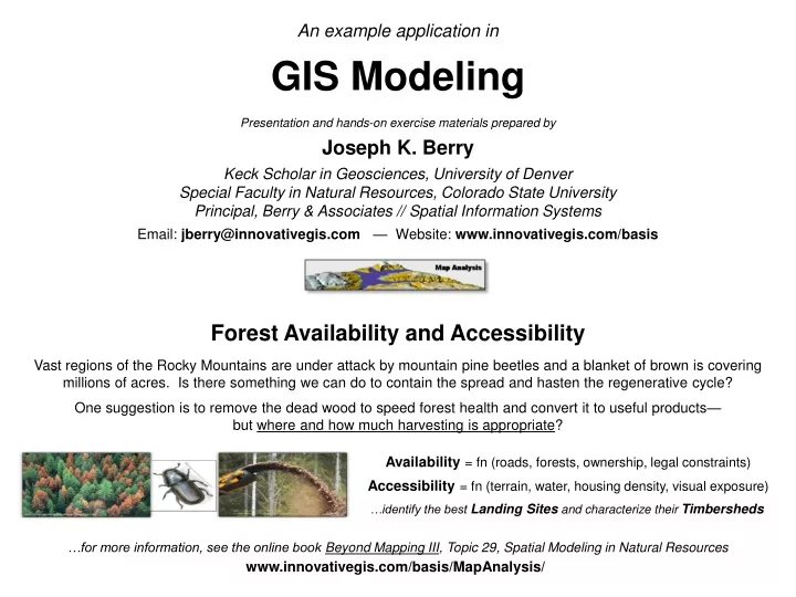
An example application in GIS Modeling Presentation and hands-on exercise materials prepared by Joseph K. Berry Keck Scholar in Geosciences, University of Denver Special Faculty in Natural Resources, Colorado State University Principal, Berry & Associates // Spatial Information Systems Email: jberry@innovativegis.com — Website: www.innovativegis.com/basis Forest Availability and Accessibility Vast regions of the Rocky Mountains are under attack by mountain pine beetles and a blanket of brown is covering millions of acres. Is there something we can do to contain the spread and hasten the regenerative cycle? One suggestion is to remove the dead wood to speed forest health and convert it to useful products— but where and how much harvesting is appropriate? Availability = fn (roads, forests, ownership, legal constraints) Accessibility = fn (terrain, water, housing density, visual exposure) …identify the best Landing Sites and characterize their Timbersheds …for more information, see the online book Beyond Mapping III, Topic 29, Spatial Modeling in Natural Resources www.innovativegis.com/basis/MapAnalysis/
Mountain Pine Beetle Devastation (Situation) Vast regions of the Rocky Mountains are under attack by mountain pine beetles. One possible action to help contain the spread of the beetles and improve forest health is to remove the dead wood… Feller Buncher Skidder Wood Chipper …but where and how much harvesting is environmentally, economically and socially appropriate? http://ndn1.newsweek.com/media/24/colorado-beetle-forest-destroy-wide-horizontal.jpg http://summitvoice.files.wordpress.com/2010/01/pine-beetle-map.jpg http://earthtrends.wri.org/images/pine_beetle_dist.jpg
Assessing Forest Availability and Access (Fundamental considerations) Roads Forests Ownership Sensitive Areas Forested areas are first assessed for Availability considering ownership and sensitive area designation… Intervening Considerations Forests and Roads …and then characterized by Relative Accessconsidering intervening terrain factors of steepness and stream buffers, plus human factors of housing density and visual exposure to roads and houses. Slope Water Houses
Forest Access Model (Flowchart) Basic Access Model Forest Access Model A map of Slope is used to establish relative and absolute barriers for operating mechanized harvesting equipment. Maps of Ownership, Water, and Sensitive Areas are used to establish additional absolute barriers based on legal constraints. Forest Accessibility 0 =road to 120+ units away Discrete Cost Surface Relative Steepness 1 = best : 9 = worst Unavailable Water Buffer = 0 Unavailable Too Steep = 0 else assigned 1 Unavailable Ownerships = 0 Ownership Water Slope Slope Sensitive Areas Unavailable Sensitive = 0 Preference 0 = no-go 1 = best : 9 = worst Relative Accessibility 0 = road location to 120+ units away Roads 1 = road 0 = no road Forests 0 = not forested 1= forested Accumulation Cost Surface Critical “ Map Variables” determining Accessible Forests locations “Effective Proximity” Processing Flowchart
Basic Model Results (Effective proximity) Accessible Forests by Effective Proximity 120 Reach 40 Reach Not Available Effectively Too Far Relative access values for all of the available forested locations with warmer tones indicating a long harvesting reach into the woods. Far Not Forested Far Simulation of different “reach scenarios” provides information on variations in wood supply from reaching deeper into the forest at increasingly higher access costs. The inset on the right shows the forested areas that are much more easily accessed (40/120= .33 as far). Note the elimination of available forested locations (yellow to red) that are deemed effectively “too far” from roads. 0 1000 2000 ft
Extended Forest Access Model (Flowchart) Basic Access Model(Physical and Legal concerns) Forest Accessibility 0 =road to 120+ units away Discrete Cost Surface Relative Steepness 1 = best : 9 = worst Unavailable Water Buffer = 0 Unavailable Too Steep = 0 else assigned 1 Unavailable Ownerships = 0 Ownership Water Slope Slope Sensitive Areas Unavailable Sensitive = 0 Preference 0 = no-go 1 = best : 9 = worst Relative Accessibility 0 = road location to 120+ units away Roads 1 = road 0 = no road Forests 0 = not forested 1= forested Accumulation Cost Surface Basic Extended Model Extended Extended Access Model(Human Concerns) …willing to reach farther into areas with low visual exposure and housing density Multiplicative Weight Roads Viewer Locations Compute Visual Exposure 0 = not seen to 344+ seen VE Adjust 1 = >75 High .7 = 20 to 75 .5 = 0 to 20 Low Renumber Radiate Houses Elevation Avg Weight 1 = High : .7 = Medium : .5 = Low Extended Model Average HD Adjust 1 = >50 High .7 = 20 to 50 .5 = 0 to 20 Low Housing Density 0 = no houses to 66+ houses Houses Renumber Scan
Comparison of Basic and Extended Model Results Basic Model Resultson the left-side indicates that the farthest away location is 116 effective distance units considering physical and legal barriers to access. Max = 116 Max = 76 Max = 116 Max = 76 Extended Model Resultson the right-side indicates that the farthest away location is 76 effective distance units when considering the preference to harvest in areas of low visual exposure and housing density.
Characterizing Accessible Forest Areas (Watershed area & timber types) 1)Create a Binary Map of Accessible Forests Relative Access Accessible Forest Template Map Watersheds Renumber Data Map Accessible Forest 2)Region-Wide Overlay Composite Vegetation Type …there are 374 acres of accessible forest in Watershed 3 Accessible Forest …there are 964 acres of accessible Lodgepole Pine Compute 3)Location-Specific Overlay
Identifying Candidate Landing Sites(Gently sloped forest roads) Stream_buffer 1) COMPUTE Roads times Forests times Unavailable times Protected times Stream_buffer for Forest_roads Forest_Roads 1 The Forest_Roads map identifies road locations passing through available forest areas. Protected Unavailable Forests Roads Roads_avgSlope Landing_candidates 0 increasing steepness 65 The Landing_candidates map identifies road locations with gentle to moderate terrain (0-15% slope) within a 100 foot reach (~one acre) of a road that is accessible to available forested areas. Slope 2 3 Forest_Roads 2) SCAN Slope Average within 1 square around Forest_roads for Forest_roads_avgSlope 3) RENUMBER Forest_roads_avgSlope assign 1 to .01 thru 15 assign 0 to 15 thru 200 for Landing_candidates
Locating the Best Landing Sites (High optimal path density) 4) COMPUTE Discrete_cost Times Forests for Dcost_forests The Accum_proximity map identifies the forest areas accessible from the Landing_Candidates as a continuous surface of effective distance. 5) SPREADLanding_candidates to 200 THRU Dcost _forests Simply for Accum_proximity Accum_proximity OptimalPath_density Landing_candidates Dcost forests Discrete_cost 6) DRAINForests over Landing_accumulated_cost for OptimalPath_density High_pathDensity Landing_clumps 7) RENUMBER OptimalPath_density assign 0 to 0 thru 40 assign 1 to 40 thru 1000 for High_pathDensity (#5, 58 paths) (#2, 256 paths) 6 4 5 8 7 9 Potential_Landings (#4, 56 paths) (#6, 155 paths) 8) COMPUTE High_pathDensity Times Landing_candidates FOR Potential_landings (#9, 407 paths) Services the largest number of accessible forest locations (#13, 159 paths) Landing _candidates 9) CLUMP Potential_landings Diagonally AT 1 FOR Landing_clumps (#15, 785 paths) The Landing_clumps map uniquely identifies the locations with the most accessible forests optimally connected
Identifying “Timbersheds” of the Best Landing Sites Landings_best Landings_Accessible_forest (#5, 58 paths) (#2, 256 paths) 10) RENUMBER Landing_clumps assign 0 to 1 assign 0 to 3 assign 0 to 7 thru 8 assign 0 to 10 thru 12 assign 0 to 14 assign 0 to 16 thru 50 for Landings_best (#4, 56 paths) (#6, 155 paths) 10 (#9, 407 paths) (#13, 159 paths) 11) SPREAD Landings_best to 200 thru D_cost_forest simply for Landings_Accessible_forest (Landing #15, 785 paths) 12) RENUMBER Landings_Accessible_forest ASSIGNING -4 TO 80 THRU 200 FOR Timbersheds Timbersheds …considering a practical reach of 80 effective cell lengths #5 #2 #4 #6 #9 11 The Timbersheds map identifies all of the accessible forest locations that are “optimally” skidded to each of the Landing sites. #13 Timbershed #15 Timbershed #15 740cells * .222ac/cell = 164 acres
Mapping involves precise placement of physical features and inventories (Discrete/Graphic) Modeling involvesanalysis of spatial relationships and patterns (Continuous/Numerical) Descriptive Mapping Prescriptive Modeling (Nanotechnology)Geotechnology(Biotechnology) …enabling technology used in spatial reasoning, dialog and decision-making— Geotechnologyis one of the three "mega technologies" for the 21st century and promises to forever change how we conceptualize, utilize and visualize spatial relationships in scientific research and commercial applications (U.S. Department of Labor) Geographic Information Systems (map and analyze) Global Positioning System (location and navigation) Remote Sensing (measure and classify) GPS/GIS/RS The Spatial Triad WhereisWhat WhyandSo What Map Analysis …provides “tools” for investigating spatial patterns and relationships
A Logical Framework for Map Analysis Geotechnology– one of three “mega-technologies” for the 21st Century Global Positioning System(Location and navigation) Remote Sensing(Measure and classify) Geographic Information Systems(Map and analyze) 70sComputer Mapping(Automated cartography) 80sSpatial Database Management(Mapping and geo-query) 90sMap Analysis (Spatial relationships and patterns) 00sMultimedia Mapping (Spatial relationships and patterns) Map Analysis Toolbox Spatial Analysis(Geographic context) Reclassify (single map layer; no new spatial information) Overlay (coincidence of two or more map layers; new spatial information) Proximity (simple/effective distance and connectivity; new spatial information) Neighbors (roving window summaries of local vicinity; new spatial information) Spatial Statistics(Numeric context) Surface Modeling (point data to continuous spatial distributions) Spatial Data Mining (interrelationships within and among maps) …for more information see www.innovativegis.com/basis/Papers/Other/GISmodelingFramework/