Download
1 / 33
330 likes | 478 Vues
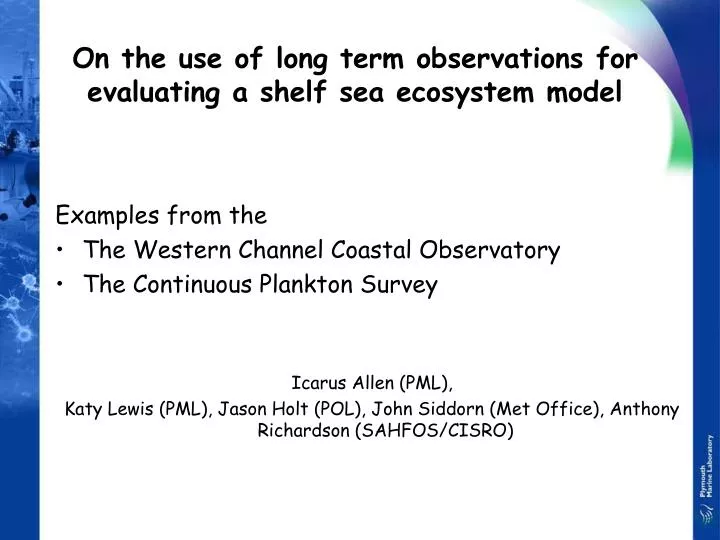
Examples from the The Western Channel Coastal Observatory The Continuous Plankton Survey Icarus Allen (PML), Katy Lewis (PML), Jason Holt (POL), John Siddorn (Met Office), Anthony Richardson (SAHFOS/CISRO). On the use of long term observations for evaluating a shelf sea ecosystem model.

E N D
Examples from the The Western Channel Coastal Observatory The Continuous Plankton Survey Icarus Allen (PML), Katy Lewis (PML), Jason Holt (POL), John Siddorn (Met Office), Anthony Richardson (SAHFOS/CISRO) On the use of long term observations for evaluating a shelf sea ecosystem model
Marine System Model: ERSEM Atmosphere CO2 O2 DMS Si Phytoplankton N u t r i e n t s Cocco- liths Pico-f Diatoms NO3 Flagell -ates Particulates DIC NH4 Bacteria PO4 Dissolved Hetero- trophs Micro- Meso- Consumers Suspension Feeders D e t r i t u s Oxygenated Layer N u t r I e n t s Aerobic Bacteria Meio- benthos Deposit Feeders Redox Discontinuity Layer Anaerobic Bacteria Reduced Layer ERSEM - key features Carbon based process model Functional group approach Resolves microbial loop and POM/DOM dynamics Complex suite of nutrients Includes benthic system Explicit decoupled cycling of C, N, P, Si and Chl. Adaptable: DMS, CO2/pH, phytobenthos, HABs. Consequently flexible and applicable to a wide range of global ecosystems. Ecosystem Forcing Cloud Cover Wind Stress Irradiation Heat Flux Physics 0D Rivers and boundaries 1D 3D UK MO GOTM POLCOMS
Shelf seas ecosystem hindcast – forecast modelling Met Forcing NWP Met Office 1/3o Atlantic FOAM model Met Office POLCOMS 12 km Atlantic Margin Model 7km MRCS POLCOMS-ERSEM Met Office 7 day hindcast 2002-pres T, S, U, V T, S, U, V POL/PML hindcast 1988/89 T, S, U, V ERSEM 7km Western Channel POLCOMS-ERSEM PML-delayed 7 day Hindcast 2002-pres
Overall Aims and Purpose: Our purpose is to integrate in situ measurements made at stations L4 and E1 in the western English Channel with ecosystem modelling studies and Earth observation. 1. What is the current state of the ecosystem? 2. How has the ecosystem changed? 3. Short term forecasts of the state of the ecosystem. 4. The WCO as a National Facility for EO algorithm development, calibration and validation: Western Channel Coastal Observatory
Western Channel Coastal Observatory • Western English Channel: • boundary region between oceanic and neritic waters; • straddles biogeographical provinces; • both boreal / cold temperate & • warm temperate organisms • considerable fluctuation of flora and fauna since records began. • Southward et al. (2005) Adv. Mar. Biol., 47
Situated 10nm south of Plymouth Sampled weekly for physical, biological and chemical data since 1992. Hydrodynamically complex Average depth of 50m; Classified as a well-mixed tidal station but it exhibits weak seasonal stratification in summer and is influenced by the outflow from the River Tamar. On some occasions it represents the margin of the tidal front characteristic of this region (Pingree, 1978). Station L4 Complex system so a good test of the model dynamics
The thermohaline structure of the water column was determined with a CTD probe developed from the Undulating Oceanographic Recorder (UOR) (Aiken & Bellan, 1990). Water samples (10m depth) analysed for nitrate, phosphate and silicate concentrations using standard laboratory colorimetric methods (Woodward & Rees, 2001). Chlorophyll-a concentrations, fluorometric analysis with a Turner Design 1000R fluorometer after extraction in 90% acetone overnight. (Rodriguez et al., 2000) Phytoplankton is collected at 10m depth and preserved with 2% Lugol’s iodine solution (Holligan & Harbour, 1977). Between 10 and 100ml of sample, depending on cell density, were settled and species abundance was determined using an inverted microscope. Cell volume and carbon estimates for the microplankton were derived from the volume calculations of Kovala & Larrance (1966) and the cell volume and carbon estimations of Eppley et al. (1970). Zooplankton samples are collected by vertical net hauls (WP2 net, mesh 200μm; UNESCO, 1968) from the sea floor to the surface and stored in 5% formalin. (Bacteria and picophytoplankton (the combination of synecoccus bacteria and picoeukaryotes)) determined using a flow cytometer. Station L4
MDS (multi-dimensional scaling) Cluster analysis allows us to check the adequacy and mutual consistency of both the model and the in-situ data. A multi-variate ordination technique which can be used to reflect configurations in the model and in-situ data A non-metric MDS algorithm constructs MDS plots iteratively by as closely as is possible satisfying the dissimilarity between samples; dissimilarities between pairs of samples, derived from normalised Euclidean-distance matrices, are turned into distances between sample locations on a map. RELATE Test. A test of ‘no relationship between distance matrices’, essentially a test for concordance in multivariate pattern. A correlation between corresponding elements in each distance matrix was calculated using Spearman’s rank correlation, adjusted for ties (Kendall, 1970). The significance of the correlation was determined by a Monte Carlo permutation procedure, using the PRIMER program RELATE. For the ideal model r =1. Multivariate Analysisall analysis's performed using PRIMER 6
MDS MDS constructed from temperature, salinity, chlorophyll, nitrate, phosphate silicate, diatom biomass, flagellate biomass, dinoflagellate biomass. Data RELATE TEST r = 0.44, p=0.0001 T,S and Nutrients only r = 0.55, p = 0.0001 Model
Correlations between variables at L4 Model Nitrate control in model to strong? Data RELATE test between these data sets indicates a statistically significant similarity between the matrices r = 0.53 p=0.012 i.e. model explains ~ 28% of observed correlations
Summary • Model does well reproducing temperature and has some skill for nutrients, but phytoplankton must be improved before any confidence can be had in the model ability to forecast. • The model does not accurately simulate the timing of the spring bloom and further work is required to assess whether the causes of this are hydrodynamic, optical or physiological. • Issues with model • Salinity and hence water column structure / turbulence • b) Grazing pressure • c) Nitrogen dynamics in phytoplankton • d) Dinoflagellate dydnamic incorrect (lack of motility / heterotrophy?) • e) Optics
Model validation with plankton abundance Qualitative Validation K. Lewis et al., Error quantification of a high resolution coupled hydrodynamic-ecosystem coastal-ocean model: Part3, validation with Continuous Plankton Recorder data, Journal of Marine Systems (2006), doi:10.1016/j.jmarsys.2006.08.001.
Continuous Plankton Surveywww.sahfos.ac.uk The aim of the CPR Survey is to monitor the near-surface plankton of the North Atlantic and North Sea on a monthly basis, using Continuous Plankton Recorders on a network of shipping routes that cover the area.
Resolving shifts in species distributions Zooplankton species geographical shift We need to be able to model this to understand how climate will affect marine bioresources
Simulated ‘tows’ were performed by extracting biomass data from archived model Due to the semi-quantitative nature of the CPR, data for each individual tow of both the CPR and corresponding model output were standardised to a mean of zero and a unit standard deviation (σ) of the relevant data to produce a dimensionless z-score. This allows a direct qualitative comparison of model biomass with discrete survey counts. Domain-wide daily mean values for all CPR samples and corresponding model output were used to compare the magnitude and timing of the behaviour of the biological variables over the two-year period.
Spatial Distribution of Errors Total Phytoplankton
% Model results month by month that differ from the CPR samples by less that 0.5 SD from the mean in 1988
Simple linear regression and absolute error maps provide a qualitative evaluation of spatio-temporal model performance z-scores indicate model reproduces the main pelagic seasonal features good correlation between magnitudes of these features with respect to standard deviations from a long-term mean. The model is replicating up to 62% of the mesozooplankton seasonality across the domain, with variable results for the phytoplankton. There are, however, differences in the timing of patterns in plankton seasonality. The spring diatom bloom in the model is too early, suggesting the need to reparameterise the response of phytoplankton to changing light levels in the model. Errors in the north and west of the domain imply that model turbulence and vertical density structure need to be improved to more accurately capture plankton dynamics. Summary
Long-term time series observations are important resources for the assessment of model performance; they can be used to highlight errors in model hindcasts, which can subsequently be improved. These types of analysis are only possible because of the existence of large self-consistent data sets. Unfortunately, such data sets are relatively rare and a concerted effort is required to collate existing data sets into model friendly formats, collect new ones and make them readily available. L4 is situated in a hydrographically complex region therefore it provides a substantial test of model ability, however for the model to be evaluated more extensively it is essential to perform these tests over a wider spatial scale. General Conclusions
Advances in Marine Ecosystem Modelling Research Workshop on ‘validation of global ecosystem models (4-6th Feb 2007) Workshop on ‘Ocean Acidifcation’ (11-13th Feb 2007) Both workshops to be held in Plymouth, register online at www.amemr.info by 17th November. AMEMR II is scheduled for June 2008.
A coherent ecosystem approach. In-Situ Data Earth Observation Meteorological Station 3D Ecosystem Modelling Web based data delivery systems