Download
1 / 55
660 likes | 1.8k Vues
Causal Diagrams: Directed Acyclic Graphs to Understand, Identify, and Control for Confounding. Maya Petersen PH 250B: 11/03/04. What is causation?. Ex: We observe a high degree of association between carrying matches and lung cancer

E N D
Causal Diagrams: Directed Acyclic Graphs to Understand, Identify, and Control for Confounding Maya Petersen PH 250B: 11/03/04
What is causation? • Ex: We observe a high degree of association between carrying matches and lung cancer • Can we infer that carrying matches causes lung cancer? • The counterfactual definition of causation: • Carrying matches is a cause of lung cancer if the risk of lung cancer is higher in people who carry matches than it would be if these exact same people did not carry matches
Causal diagrams • Intuitive approach to representing our assumptions about causal relationships • Provide relatively straightforward tool for relating observed statistical associations and causal effects • What do we need to know (or assume) before we can infer that an exposure causes a disease, and get an unbiased estimate of this effect?
Causal diagrams • Today will focus on • How to draw a causal diagram • Use of causal diagrams to decide: • Is confounding present? • What should we adjust for to get an unbiased estimate of effect? • Causal diagrams to illustrate a situation where the traditional approach to controlling confounding (i.e. multivariable adjustment) fails
Ex . Constructing a Causal Diagram • We are interested in the effect of maternal multivitamin use on birth defects, and make the following causal assumptions: • Prenatal care (PNC) leads to an increase in vitamin use (as a result of intervention and education.) • Prenatal care protects against birth defects in ways other than by increasing vitamin use . • Difficulty conceiving may cause a woman to seek out PNC once she becomes pregnant • Maternal genetics that lead to difficulty conceiving can also lead to birth defects. • Socio-economic characteristics directly affect both access to PNC and use of vitamins
Ex: Constructing a Causal Diagram Difficulty conceiving SES Maternal genetics Pre-Natal Care Vitamins Birth Defects
Directed Acyclic Graph (DAG) construction: Basics • Direct causal relationships between variables are represented by arrows • All causal relationships have a direction, because any given variable cannot be simultaneously a cause and an effect (Directed) • There are no feedback loops ( Acyclic) • There can be no feedback loops because causes always precede their effects • To avoid feedback loops, extend graph over time Malnutrition Malnut. (t=0) Malnut. (t=1) Infection Infect. (t=0) Infect. (t=1)
Directed Acyclic Graph (DAG) construction: Terminology • Parent & Child: • Directly connected by an arrow (No intermediates) • Pre-Natal care is a “parent” of birth defects • Birth defects is a “child” of Pre-natal care • Ancestor & Descendant: • Connected by a directed path of a series of arrows • SES is an “ancestor” of Birth Defects • Birth Defects is a “descendant” of SES Difficulty conceiving SES Maternal genetics Pre-Natal Care Vitamins Birth Defects
Directed Acyclic Graph (DAG) construction: Assumptions • Not all intermediate steps between two variables need to be represented (depends on level of detail of the model) • Ex: can represent the effect of smoking on lung cancer as: Smoking -> Cancer or Smoking -> tar -> mutations -> Cancer • Absence of a directed path from X to Y implies that X has no effect on Y
Directed Acyclic Graph (DAG) construction: Assumptions • DAGs assume that all common causes of exposure and disease of interest are included in causal diagram • If common causes are unknown, or cannot be observed, they must still be included • Ex: Unmeasured characteristics (religious beliefs, culture, lifestyle, etc.) Alcohol Use HeartDisease Smoking
Ex: What assumptions does the DAG we constructed make? • SES has no effect on difficulty conceiving • Difficulty conceiving has no effect on maternal vitamin use, other than through its effect on seeking prenatal care • SES has no effect on birth defects other than via its effects on access to prenatal care and on vitamin use • There are no additional common causes of vitamin use and birth defects • Etc… Difficulty conceiving SES Maternal genetics Pre-Natal Care Vitamins Birth Defects
Back to our basic problem: What can we say about causal effects, based on the associations we observe in our data? • Associations between exposure and disease in our crude data can arise in several ways
Crude (unadjusted) associations in our observational data:1) Exposure causes disease • A crude association between smoking and cancer could be due to • Smoking -> Cancer • Smoking -> tar -> mutations -> Cancer • Adjusting for an intermediate in the causal pathway between exposure and disease removes any association that results from that pathway • In the DAG above, if we control for tar levels, we will block the association between smoking and cancer Smoking tar mutations Cancer • By adjusting for the effects of the exposure, we will no longer be able to study them
Crude (unadjusted) associations in our observational data:2)Exposure and disease share a common cause • A crude association between matches and cancer could be due to • Matches have no causal effect on cancer, but the two are associated because they have a common cause (smoking) • This is a classic example of confounding • By adjusting for the common cause, association is eliminated • Matches are no longer associated with cancer after we stratify on smoking • This is what we do when we adjust for a confounder Smoking Matches Cancer
Yet again- What is confounding? • If the crude association between exposure and disease is unconfounded, then • All of the association we see between exposure and disease is due to the effect of exposure on disease • None of the association between exposure and disease is due to common causes that they share. (confounding) • In other words: If exposure has no effect on disease, would we still expect to observe an association in our data? • If yes -> confounding is present
How can we use a DAG to check for presence of confounding? • Remove all direct effects of the exposure • These are the effects we are interested in. We want to see if, in their absence, an association is still present. • Check whether disease and exposure share a common cause (ancestor) • Does any variable connect E and D by following only forward pointing arrows? • If E and D have a common cause -> confounding is present • Any common cause they share will lead to an association between E and D that is not due to the effect of E on D
Vitamins and Birth Defects Is confounding present? • Remove all direct effects of vitamin use • Do exposure and disease share a common cause (ancestor)? SES Difficulty conceiving Maternal genetics Pre-Natal Care Vitamins Birth Defects
How can we use a DAG to decide what variables to control for in our analysis? • We want to choose a set of variables that, when adjusted for, will give us an unconfounded estimate of the effect of exposure on disease • In other words, if the exposure had no effect on disease, after adjusting for these variables, exposure and disease will no longer be associated
How can two variables become associated? • Review: A crude (unadjusted) association between exposure (E) and disease (D) can be due to • Causal pathway from E to D (or vice versa) E -> DorE -> x -> y -> D • Common cause of E and D • By adjusting (or stratifying) on a third variable, it is possible to introduce a new source of non-causal association (confounding) between E & D • As we begin to adjust for variables in attempt to control for confounding, we must take this potential source of association into account C E D
Adjusting for a common effect of two variables will induce a new association between them (Even if they were unassociated before adjusting) • Ex: • Being on a diet does not cause cancer (or vice versa), and dieting and cancer share no common causes: In our crude data, diet and cancer will not be associated • Whether or not an individual was on a diet does not tell us anything about whether or not he/she has cancer. • If we stratify on weight loss, we can create a new association between dieting and cancer • Within the strata of people who lost weight, if we know an individual was on a diet, it tells us that he/she is less likely to have cancer (dieting provides an alternate explanation for weight loss). Weight-loss diet Cancer Weight Loss
Using a DAG to decide what variable to adjust for in analysis Ex 1: Is adjusting for prenatal care sufficient to control for confounding of the effect of vitamin use on birth defects?
Using a DAG to decide what to adjust for in analysis • Step 1: Is prenatal care caused by vitamin use? If yes, we should not adjust for it. • Do not adjust for an effect of the exposure of interest SES Difficulty conceiving Pre-Natal Care Maternal genetics Vitamins Birth Defects
Using a DAG to decide what to adjust for in analysis • Step 2: Delete all non-ancestors of vitamin use, birth defects, and pre-natal care • If a variable is not an ancestor of vitamin use or birth defects, it cannot be a common cause, and so cannot be a source of crude association between them • If a variable is not an ancestor of prenatal care, new associations with that variable can not be created by adjusting for prenatal care Difficulty conceiving SES Maternal genetics Pre-Natal Care Vitamins Birth Defects
Using a DAG to decide what to adjust for in analysis • Step 3: Delete all direct effects of Vitamins • These are the effects we are interested in. We want to see if, in their absence, an association is still present. If it is, we still have confounding. SES Difficulty conceiving Pre-Natal Care Maternal genetics Vitamins Birth Defects
Using a DAG to decide what to adjust for in analysis • Step 4: Connect any two causes sharing a common effect • Adjustment for the effect will result in association of its common causes SES Difficulty conceiving Pre-Natal Care Maternal genetics Vitamins Birth Defects
Using a DAG to decide what to adjust for in analysis • Step 5 : Strip arrow heads from all edges • We are moving from a graph that represents causal effects, to a graph that represents the associations we expect to observe (as a result of both causal effects and the adjustment process) SES Difficulty conceiving Pre-Natal Care Maternal genetics Vitamins Birth Defects
Using a DAG to decide what to adjust for in analysis • Step 6 : Delete prenatal care • This is equivalent to adjusting for prenatal care, now that we have added to the graph the new associations that will be created by adjusting SES Difficulty conceiving Maternal genetics Vitamins Birth Defects
Using a DAG to decide what to adjust for in analysis • Test: Are Vitamins and Birth Defects still connected? • Yes: Adjusting for Prenatal Care is not sufficient for control of confounding • After adjusting for prenatal care, vitamin use and birth defects will still be associated in our data, even if vitamin use has no causal effect on birth defects Difficulty conceiving SES Maternal genetics Vitamins Birth Defects
Using a DAG to decide what to adjust for in analysis • Adjustment for which variables would result in control of confounding? • Our DAG shows that adjusting for any one or more of the three remaining variables, in addition to prenatal care, would be sufficient for control of confounding(e.g.SES and prenatal care) Difficulty conceiving Maternal genetics Vitamins Birth Defects
Vitamins and Birth Defects: Lessons learned • It may not be immediately intuitive what variables we need to control for in our analysis • The process of adjustment/stratifiction can introduce new sources of association in our data that must be accounted for in any attempt to control confounding • Step by step analysis of a DAG provides a rigorous check whether we have adequately controlled for confounding • Adjustment for several different sets of confounders may each be sufficient to control confounding of the same exposure disease relationship. • Can inform study design
DAGs for control of confounding: Summary of Steps Problem: Is adjustment for/stratification on a set of confounders “C” sufficient to control for confounding of the relationship between E and D? • No variables in C should be descendants of E • Delete all non-ancestors of {E, D, C} • Delete all arrows emanating from E • Connect any two parents with a common child • Strip arrowheads from all edges • Delete C Test: If E is disconnected from D in the remaining graph, then adjustment for C is sufficient to remove confounding Pearl, J. Causality. Cambridge University Press, Cambridge UK. 2001. pp. 355-57.
Stratification has its limits… • Up till now, you have heard about one way to remove confounding: adjustment or stratification on certain variables • But… in some situations, there are no variables you can stratify on and sucessfully remove confounding • We will illustrate this using a DAG • In a future lecture, you will hear about a method you can use in these circumstances (Marginal Structural Models)
A DAG-based illustration of time-dependent confounding:A situation in which traditional methods to control for confounding (i.e. adjustment/stratification) break down Ex: What variables should we control for to estimate the effect of antiretroviral therapy on CD4 count?
Ex.: Antiretroviral therapy and CD4 count • Question of interest: What is the effect of antiretroviral therapy on CD4 count? • Study Population: A cohort of HIV-infected individuals • Outcome: CD4 count at the end of the study • Exposure: Antiretroviral therapy (ART) (treated or not for the entire study period)
Ex. : Antiretroviral therapy and CD4 count • Sicker individuals (those with lower baseline CD4 counts at the beginning of the study) are more likely to be treated with ART • Low baseline CD4 count causes physicians to treat their patients • CD4 count at baseline also affects CD4 count at the end of the study
Representing these relations in a DAG CD4 Count at beginning of study Outcome: CD4 count at the end of a study Causal effect of interest Exposure: Antiretroviral Treatment
Simple confounding • CD4 count at baseline is a confounder • If we don’t adjust for baseline CD4 count, we will underestimate the effect of ART on preserving final CD4 count • Sicker people/ those with lower initial counts will be overrepresented among those who get treated • We can see this in the DAG- we must adjust for baseline CD4 or ART and final CD4 will still be connected once we delete our causal effect of interest • CD4 and ART share a common cause
Representing these relations in a DAG Confounder CD4 Count at beginning of study Outcome: CD4 count at the end of a study Exposure: Antiretroviral Treatment
Antiretroviral therapy and CD4 count: A more realistic example • Same study population and outcome • Cohort of HIV-infected • Outcome is final CD4 count • Now, an individual can change treatment status during the course of follow-up • E.g. an individual who is not treated at the beginning of the study (t=0) may go on treatment partway through the study (e.g. t=1) • CD4 also measured during course of follow-up
DAG- Expanded to incorporate changing treatment over time Baseline confounder Y: Final CD4 count CD4 Count at beginning of study (t=0) CD4 Count partway through study (t=1) Causal effect of interest Antiretroviral Treatment at t=0 Antiretroviral Treatment at t=1
Something is missing…. • Our effect of interest is how antiretroviral treatment throughout the study (eg t=0 and t=1) affects final CD4 count • We have left out an important causal relationship in the previous DAG! • Antiretroviral treatment at baseline affects intermediate CD4 counts (e.g. CD4 measured at t=1) , which in turn affect final CD4 counts • This is part of our causal effect of interest!
Filling in the DAG Baseline confounder Y: Final CD4 count CD4 Count at beginning of study (t=0) CD4 Count partway through study (t=1) Causal effect of interest Antiretroviral Treatment at t=0 Antiretroviral Treatment at t=1
Something is still missing… • CD4 count at t=1 will also affect subsequent treatment (ART at t=1) • Note: we take the convention that CD4(t) is measured before ART(t) • Patients with lower CD4 counts at t=1 are more likely to start ART partway through the study • A patient getting sicker causes his/her physician to start them on treatment
Filling in the DAG Baseline confounder Y: Final CD4 count CD4 Count at beginning of study (t=0) CD4 Count partway through study (t=1) Causal effect of interest Antiretroviral Treatment at t=0 Antiretroviral Treatment at t=1
What does this DAG tell us about what we need to adjust for to control confounding?
Using the DAG to decide what we need to control for • We can’t adjust for anything that is a descendant of (caused by) ART • Rules out CD4 at t=1 • Delete all non-ancestors of exposure, disease, and things we are considering adjusting for • NA: Everything in current graph is an ancestor of outcome or exposure Y: Final CD4 count CD4 Count at beginning of study (t=0) CD4 Count partway through study (t=1) Causal effect of interest Antiretroviral Treatment at t=0 Antiretroviral Treatment at t=1
Using the DAG to decide what we need to control for • Delete any arrows from ART • Connect parents sharing a common child • NA: Already connected Y: Final CD4 count CD4 Count at beginning of study (t=0) CD4 Count partway through study (t=1) Antiretroviral Treatment at t=0 Antiretroviral Treatment at t=1
Using the DAG to decide what we need to control for • Strip arrowheads • What can we delete that will leave ART and final CD4 unconnected? • Remember: CD4 at t=1 is not an option since ART at t=0 affects it Y: Final CD4 count CD4 Count at beginning of study (t=0) CD4 Count partway through study (t=1) Antiretroviral Treatment at t=0 Antiretroviral Treatment at t=1
A Dilemma • From our analysis of the DAG it is clear that if we don’t adjust for CD4 at t=1, we fail to control for confounding • But we know we cannot adjust for a variable affected by our exposure of interest • Adjusting for CD4 at t=1 would be equivalent to adjusting for part of our causal effect of interest • We would again fail to correctly estimate the total effect of ART on final CD4 because we would lose that component of the effect mediated by early changes in CD4
Adjusting for a variable on the causal pathway of interest Baseline confounder- could include it in traditional multivariable model Time-dependent confounder Y: Final CD4 count CD4 Count at beginning of study t=0 CD4 Count partway through study t=1 Causal effect of interest Antiretroviral Treatment at t=0 Antiretroviral Treatment at t=1