V10: Proteome during the Yeast Cell Cycle

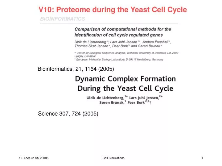
V10: Proteome during the Yeast Cell Cycle Bioinformatics, 21, 1164 (2005) Science 307, 724 (2005) Cell Simulations

Idea Well known: certain genes are expressed only at specific stages of the cell cycle, e.g. the cyclins and the histone.  these genes exhibit a periodic pattern of expression when monitored during consecutive cell cycles. Many microarry experiments have characterized the expression levels. Post-analysis by computational methods  yeast contains ca. 300 – 800 genes that are periodically expressed. Problem: results correlate very poorly, particularly when different computational methods are applied to the same data. Altogether, 1800 genes have been proposed to be expressed periodically, which is almost one third of the S. cerevisae genome. Bioinformatics, 21, 1164 (2005) Cell Simulations

Comparison of methods Benchmark different methods on three data sets: B1 113 genes identified as periodically expressed in small-scale experiments B2 Genes whose promoters are bound (p-value < 0.01) by at least one of nine known cell cycle transcription factors in two IP studies.  352 genes of which many should be cell cycle regulated B3 genes annotated in MIPS as „cell cycle and DNA processing“ Understand strengths and weaknesses of different methods. Bioinformatics, 21, 1164 (2005) Cell Simulations

Methods of analysis: statistical test for regulation The standard deviation can be easily calculated for each logratio profile, giving a measure of the spread of the samples around the mean. Heavily regulated genes will thus have large standard deviations, whereas genes without significant regulation display little deviation from the mean. To test for the significance of regulation, we therefore compare the observed standard deviation for each expression profile to a randomly generated background distribution. 1,000,000 random profiles were constructed by selecting at each time point the log-ratio from a randomly chosen gene. A p-value for regulation was calculated as the fraction of the simulated profiles with standard deviations equal to or larger than that observed for the real expression profile. Bioinformatics, 21, 1164 (2005) Cell Simulations

Methods of analysis: statistical test for periodicity To estimate a p-value for periodicity, we compared the Fourier score of the observed gene expression profile for each gene to those of random permutations of the same gene. For each gene, i, a Fourier score, Fi, was computed as where and T is the interdivision time. Similarly, scores were calculated for 1,000,000 artificial profiles constructed by random shuffling of the data points within the expression profile of the gene in question. The p-value for periodicity was calculated as the fraction of artificial profiles with Fourier scores equal to or larger than that observed for the real expression profile. The p-value for regulation is thus a comparison between individual genes and the global distribution, whereas the pvalue for periodicity is a comparison involving only data from the gene in question. Cell Simulations

Combined test for regulation and periodicity For each gene, a combined p-value of regulation was calculated by multiplying the separate p-values of regulation from each of the three experiments. Analogously, a combined p-value of periodicity was calculated. Subsequently, the p-value of regulation and p-value of periodicity were multiplied to obtain the total p-value. An undesirable feature of the total p-value is that it may become very low (i.e. highly significant) due to only one of the tests. Genes that are strongly regulated but not periodic (or vice versa) will thus receive good scores. To address this, we multiply the total p-value with two penalty terms that weight down genes that are either not significantly regulated or not significantly periodic. The final score used for ranking is: Bioinformatics, 21, 1164 (2005) Cell Simulations

Assigning the time of peak expression Since we approximate each expression profile by a sine wave, the time of peak expression for a gene in a single experiment is trivially defined as the time where the sine wave is maximal. We refer to this as the peak time. Due to differences in experimental conditions, the time it takes the cell to complete a cycle (the interdivision time) varies greatly between the alpha, Cdc15 and Cdc28 experiments. In order to compare the timing of peak expression across experiments, we therefore transformed the time-scales from minutes to percent of the cell cycle by dividing with the interdivision times estimated by Zhao et al. (2001). Combining peak times from different experiments into one is a non-trivial task, since the assignment should not be trusted in those experiments where the expression profile is not sufficiently periodic. To compensate for this, we weighted the individual peak times when computing the global, combined peak time. Bioinformatics, 21, 1164 (2005) Cell Simulations

Methods (1) M1 Cho et al. (1998) visually inspected the expression profiles of all genes regulated more than two-fold during the Cdc28 experiment, classifying 421 of them as “periodic”. M2 Spellman et al. (1998) computed a score for every gene that was based partly on the correlation to one of five idealized gene profiles, and partly on a Fourier-like score yielding the signal strength at a period similar to the interdivision time. The genes were ranked based on their combined score and truncated to 800 genes as this corresponds to a sensitivity of 90% on B1. M3 Johansson et al. (2003) used partial least squares regression to analyze the three data sets individually and in combination. The approach was based on fitting of sine curves and thus also yields an estimate of the time of peak expression. Thresholds were estimated based on random permutations of the data. Bioinformatics, 21, 1164 (2005) Cell Simulations

Methods (2) M4 Zhao et al. (2001) reanalyzed each of the three data sets individually using a statistical single–pulse model. The resulting score, describing how well a profile fits the model, is independent of the magnitude of regulation. An appealing feature of the model is that it also estimates the time of activation and deactivation of the gene. M5 Luan & Li (2004) used a modeling approach based on cubic splines, rather than sine waves. The sets were analyzed individually and the statistical nature of the method enabled the authors to identify thresholds that satisfied a given false discovery rate. M6 Lu et al. (2004) used Bayesian modeling techniques to estimate a periodic–normal mixture model based on five microarray time courses. The authors provide a ranked list of 822 genes based on all five data sets. Bioinformatics, 21, 1164 (2005) Cell Simulations

Combination method In addition to the methods M1–M6, we also include a new and simple statistical approach (M7) based on permutations. Its score is composed of two terms: one quantifies only the magnitude of regulation, whereas the other measures the periodicity of the expression profile. The combined score ensures that high ranking genes are both significantly regulated and periodic. Bioinformatics, 21, 1164 (2005) Cell Simulations

Comparison of published methods Bioinformatics, 21, 1164 (2005) Cell Simulations

Regulation vs. periodicity Bioinformatics, 21, 1164 (2005) Cell Simulations

Agreement across experiments An alternative strategy for evaluating the performance of methods for extracting periodically expressed genes is to examine the overlap in genes identified in different experiments. For each of the methods that provide a ranked list of genes for each individual experiment, top 300 lists were extracted and their overlap visualized as Venn diagrams (see Figure 3). The results are consistent with those obtained from the benchmark sets. The results of M4, a representative of the magnitude-independent methods, shows by far the least agreement between the three experiments. In comparison, M3 and M7 identify almost twice as many genes that agree in all three experiments. For all computational methods, the alpha factor experiment shows the best overlap with the two other experiments, while the Cdc28 experiment overlaps the least. This supports our previous observations with regard to the quality of the individual experiments. The lower right Venn diagram in Figure 3 illustrates that a renormalization of the Cdc28 data improves the agreement with the two other experimental data sets, in addition to improving performance on the benchmark sets (Figure 2). When including the renormalized Cdc28 data in our analysis, two thirds of the genes detected from the alpha factor synchronization are confirmed by at least one other experiment. Bioinformatics, 21, 1164 (2005) Cell Simulations

Consistency of peak expression So far, we have addressed the issues of finding periodically expressed genes and asked if the same genes are identified in different experiments. It is, however, equally important to check that those genes behave similarly across experiments, i.e. that their expression profiles peak at the same stage in the cell cycle. As a consequence of differences in experimental protocols, the interdivision time varies between experiments. Furthermore, the synchronization methods release cells at different points in the cycle. To enable cross-experiment comparisons, we represent time in percent of the cell cycle (0% being the time of cell division) and align the time axes of the experiments relative to each other. For each gene, we can thus assign a time of peak expression in each experiment and compare these across experiments. To examine the degree of consistency between these peak times in different experiments, we computed the largest peak time difference for each gene. Figure 4 shows the distribution of these differences for the set of 89 genes that were identified as periodic in all three experiments (see Figure 3). For 87 of the 89 genes, all three peak times fall within an interval of 15% of a cell cycle, clearly demonstrating the reproducibility of peak expression by different synchronization methods. For genes that appear periodic in all three experiments, an average peak time could easily be computed. Bioinformatics, 21, 1164 (2005) Cell Simulations

Expression of phase-specific genes As a final check of the reproducibility, we investigated the timing of peak expression for four sets of known phase specific genes across the three experiments. B1 was subdivided by Spellman et al. (1998) into phase-specific groups according to their reported peak expression in the small scale experiments. The distribution of peak times within each group is visualized in Figure 5, along with the distribution of our combined peak times. From this, it is clear that the phases occur in the same order, with the same length, and at the same time in all three experiments. It thus appears that the synchronization methods cause no abnormalities of the cell-cycle transcriptional program. Together, Figures 4 and 5 show that the combined peak time is a meaningful measure that accurately describes when in the cell cycle a gene is expressed. Bioinformatics, 21, 1164 (2005) Cell Simulations

Conclusions Most surprisingly, the benchmark analysis reveals that most of the new and more mathematically advanced methods for identifying periodically expressed genes perform considerably worse than the early method by Spellman et al. (1998) (M2). These results should encourage developers of future computational methods to evaluate the performance of their methods carefully. We show that the performance gap is due to the magnitude-independence of most newer methods. This independence may improve their ability to discover novel weakly regulated cell cycle genes, however, as the magnitude of regulation contains a large part of the signal, this should be exploited in order to derive the most accurate set of cell cycle regulated genes. Using the periodicity score alone yields results similar to those of other magnitude-independent methods, while our combined score performs as well as the best existing methods. In comparison to other methods, ours have two main advantages. First, genes ranked high on our list are guaranteed to be both significantly regulated and significantly periodic. Second, we require consistency in peak time across experiments, which allows us to assign a time of peak expression to each gene. Bioinformatics, 21, 1164 (2005) Cell Simulations

Analysis of complexome during cell cycle Most research on biological networks has been focused on static topological properties, describing networks as collections of nodes and edges rather than as dynamic structural entities. Here this study focusses on the temporal aspects of networks, which allows us to study the dynamics of protein complex assembly during the Saccharomycescerevisiae cell cycle. The integrative approach combines protein-protein interactions with information on the timing of the transcription of specific genes during the cell cycle, obtained from DNA microarray time series shown before.  a quality-controlled set of 600 periodically expressed genes, each assigned to the point in the cell cycle where its expression peaks. Science 307, 724 (2005) Cell Simulations

Data preparation Construct physical interaction network for the corresponding proteins from Y2H screens, TAP pull-downs, and curated complexes from the MIPS database. To reduce the error rate of 30 to 50% expected in most current large-scale interaction screens, all physical interaction data were combined, a topology-based confidence score was assigned to each individual interactions as in the STRING database, and only high-confidence interactions were selected. These were further filtered with information on subcellular localization to exclude interactions between proteins annotated to incompatible compartments; no curated MIPS interactions were lost because of this filtering. The topology-based scoring scheme, filtering, and extraction criteria reduced the error rate for interactions by an order of magnitude to only 3 to 5%. Science 307, 724 (2005) Cell Simulations

E.g. compatible subcellular localizations Science 307, 724 (2005) Cell Simulations

Construct of temporal network Include in the extracted network (Fig. 1), in addition to the periodically expressed („dynamic“) proteins, constitutively expressed („static“) proteins that preferentially interact with dynamic ones. The resulting network consists of 300 proteins (Fig. 1, inside circle), including 184 dynamic proteins (colored according to their time of peak expression) and 116 static proteins (depicted in white). For 412 of the 600 dynamic proteins identified in the microarray analysis, no physical interactions of sufficient reliability could be found (Fig. 1, outside circle). Some may be missed subunits of stable complexes already in the network; the majority, however, probably participate in transient interactions, which are often not detected by current interaction assays. Science 307, 724 (2005) Cell Simulations

Temporal protein interaction network in yeast cell cycle Cell cycle proteins that are part of complexes or other physical interactions are shown within the circle. For the dynamic proteins, the time of peak expression is shown by the node color; static proteins are represented as white nodes. Outside the circle, the dynamic proteins without interactions are positioned and colored according to their peak time. Science 307, 724 (2005) Cell Simulations

Agreement with know complexes; error estimates de Lichtenberg et al. „cell cycle" was constructed by applying the entire scheme to „all". The MIPS complexes were not included for this analysis. de Lichtenberg et al. „all" contains the union of the Y2H screens by Uetz et al. and Ito et al. and the matrix representations of the two complex pull-down experiments by Gavin et al. and Ho et al. This interaction set is the raw data for which the error rate has been estimated to be 30-50%. de Lichtenberg et al. „45%" and „85%“consists of the subset of „all" to which we assign a topology-based quality score of at least 0.45 or 0.85, corresponding to the cutoff for including an interaction between two cell cycle proteins in the nal network (Figure 1). Interactions were not fitered based on subcellular localization data. Science 307, 724 (2005) Cell Simulations

Interpretation Virtually all complexescontain both dynamic and static subunits (Fig. 1), the latter accounting for about half of the direct interaction partners of periodically regulated proteins through all phases of the cell cycle (Fig. 2). Transcriptional regulation thus influences almost all cell cycle complexes and thereby, indirectly, their static subunits. This implies that many cell cycle proteins cannot be identified through the analysis of any single type of experimental data but only through integrative analysis of several data types. In addition to suggesting functions for individual proteins, the network (Fig. 1) indicates the existence of entire previously unknown modules. Science 307, 724 (2005) Cell Simulations

Just-in-time synthesis vs. just-in-time-assembly Transcription of cell cycle–regulated genes is generally thought to be turned on when or just before their protein products are needed: often referred to as just-in-time synthesis. Contrary to the cell cycle in bacteria, however, just-in-time synthesis of entire complexes is rarely observed in the network. The only large complex to be synthesized in its entirety just in time is the nucleosome, all subunits of which are expressed in S phase to produce nucleosomes during DNA replication. Instead, the general design principle appears to be that only some subunits of each complex are transcriptionally regulated in order to control the timing of final assembly. Science 307, 724 (2005) Cell Simulations

Interpretation Several examples of this just-in-time assembly (rather than just-in-time synthesis) are suggested by the network, including the prereplication complex (Fig. 3B), complexes involved in DNA replication and repair, the spindle pole body, proteins related to the cytoskeleton, and numerous smaller complexes or modules.  the transcriptome time mappings visualized in Fig. 1 are in close agreement with previous studies on the dynamic formation of individual protein complexes, suggesting that the timing of transcription of dynamic proteins is indicative of the timing of assembly and action of the complexes and modules (Fig. 3). Science 307, 724 (2005) Cell Simulations

Interpretation Just-in-time assembly would have an advantage over just-in-time synthesis of entire complexes in that only a few components need to be tightly regulated in order to control the timing of final complex assembly. This would explain the recent observation that the periodic transcription of specific cell cycle genes is poorly conserved through evolution. For the prereplication complex, exactly this variation between organisms has been shown, although the subunits and the order in which they assemble are conserved. Science 307, 724 (2005) Cell Simulations

Interactions during the cell cycle The number of interactions of dynamic proteins with other dynamic proteins (dynamic – dynamic) and with static proteins (dynamic – static) is shown as a function of cell cycle progression. Zero time corresponds to the time of cell division. The large number of interactions during G1 phase reflects a general overrepresentation of genes expressed in this part of the cell cycle. Science 307, 724 (2005) Cell Simulations

Dynamic modules Each panel shows a specific module from the network in Fig. 1 using the corresponding colors of individual proteins. Science 307, 724 (2005) Cell Simulations

Dynamic modules Previously unknown module connecting processes related to chromosome structure with mitotic events in the bud. The nucleosome assembly protein Nap1p is know to shuttle between the nucleus and cytosol and regulates the activity of Gin4p, one of two G1-expressd budding-related kinases in the module. Nap1p and the histone variant Htz1p connect the module to the nucleosome and sister chromatid modules, respectively. Two poorly characterized proteins, Nis1p and the putative Cdc28p substrate Yol070p are both expressed in mitosis and localize to the bud neck. Science 307, 724 (2005) Cell Simulations

Dynamic modules Schematic representation of the dynamic assembly of the prereplication complex. It contains six static proteins (Orc1p to Orc6p) that are bound to origins of replication throughout the entire division cycle. A subcomplex of six Mcm proteins is recruited to the ORC complex in G1 phase by a Cdc6p-dependent mechanism. We see the corresponding genes (except MCM6) transcribed just before that. Final recruitment of the replication machinery is dependent on Cdc45p, which is found expressed in early S phase. Science 307, 724 (2005) Cell Simulations

Dynamic modules Cdc28p module, with the different cyclins and interactors placed at their time of synthesis. At the end of mitosis, the cyclins are ubiquitinated and targeted for destruction by APC and SCF, reflected in the network by the interaction between Cdh1p and Clb2p. The latter also interacts with Swe1p, which inhibits entry into mitosis by phosphorylating Cdc28p in complex with Clb-type cyclins. In this well-studied module, an uncharacterized protein, Ypl014p, was discovered as well. Science 307, 724 (2005) Cell Simulations

Timing of expression for interaction partners The distribution of time differences between dynamic interaction partners reveals a strong preference for interactions between proteins expressed close in time. Science 307, 724 (2005) Cell Simulations

Timing of expression for interaction partners For each hub protein, the average difference in peak time was calculated among the dynamic interaction partners. The distribution is bimodal, supporting the proposition of two classes of hubs, namely „party“ and „date“ hubs. Representative hub proteins are marked in the figure to illustrate the relation between the two types of hubs and modules. Science 307, 724 (2005) Cell Simulations

Outlook With the emergence of new large-scale data sets, including assays focused on protein-DNA interactions and transient protein-protein interactions, we expect more of the dynamic proteins to be included in the network. Also, we currently lack information about the life- time of the observed complexes and modules. With reliable time series of protein abundances, preferably in individual compartments, the resolution of this temporal network can be increased considerably, because even individual interactions over time could then be monitored. Moreover, the integrative approach presented here should be applicable to any biological system for which both interaction data and time series are available. Science 307, 724 (2005) Cell Simulations

V10: Proteome during the Yeast Cell Cycle