Download

1 / 91
930 likes | 1.28k Vues
Traffic Flow models for Road Networks. Presented By Team 2. OUTLINE. Motivation Introduction Problem statement Classification Related work Microscopic models Macroscopic models Mesoscopic models Comparison Future work Conclusion. MOTIVATION.

E N D
Traffic Flow models for Road Networks Presented By Team 2
OUTLINE • Motivation • Introduction • Problem statement • Classification • Related work • Microscopic models • Macroscopic models • Mesoscopic models • Comparison • Future work • Conclusion
MOTIVATION • Traffic congestion is a serious problem, that we have to deal with in order to achieve smooth traffic flow conditions in road networks. • Also expanding infrastructure of road networks such as widening the roads was just not sufficient to handle the smooth traffic flow conditions in road networks due to increased traffic demands
INTRODUCTION • Traffic congestion is one of the major problems affecting the whole world • Intelligent transportation systems like ATMS and ATIS face a big challenge in controlling traffic congestion and estimating the traffic flow in road networks. • To model efficient Traffic flow in road networks, clear understanding on traffic flow operations like what causes congestion, how congestion propagation takes place in road networks etcare required • Many traffic flow theories and models have been devoloped in this context
Contd… • This made us to survey some traffic flow models for road networks • In our presentation we are going to explain some traffic flow models, their classification and their applications in the road network.
Problem statement • Intelligent transportation systems like ATMS and ATIS face a big challenge in controlling traffic congestion and estimating the traffic flow in road networks. • A need for some traffic flow modelling methods to control the congestion in urban , free way as well as at the intersection areas.
classification • Traffic flow models classified in many ways based on 1. Level of details • Macroscopic • Mesoscopic and • Microscopic traffic flow models 2. Operationalization criteria • Simulation • Analytical 3. Representation of processes • Stochastic • Deterministic 4.Time scale • Discrete • Continuous .
Contd… But our research just classifies the traffic flow models based on their level of detail as shown below Traffic flow models Microscopic Mesoscopic Macroscopic Cell Automation Model Car following Model AMS UTN DTA LWR
Microscopic Traffic Flow Model • A microscopic simulation model describes both the space time behaviour of the systems entities( vehicles and drivers) as well as their interactions at a high level of detail(individually). • Two types of Microscopic traffic flow model i)Car Following Model ii)Cell Automation Model
Definiton • In the car-following theory, the relation between the preceding vehicle and the following vehicle is described that each individual vehicle always decelerates or accelerates as a response of its surrounding stimulus. Therefore, the nth vehicle’s motion equation can be summarized as follows [Response]n∝ [Stimulus]n • The stimulus may include the velocity of the vehicle, the acceleration of the vehicle, the relative velocity and spacing between the nth and n+1th vehicle (the nth vehicle follows the n+1th vehicle).
RELATED WORK • Limitations of both the psycho-physical spacing model and of fuzzy models seem less than safe distance models and the stimulus-response mode. • The Collision avoidance (CA) model is also called the safety distance model. • According to the model, collision would be unavoidable if the distance is shorter than the safe distance and the behavior of the preceding vehicle is unpredictable. • Simple models that have one or few functions, such as the safe distance and stimulus-response models, cannot describe certain traffic phenomena.
Proposed Car following model • First, the model should describe certain traffic flow phenomena. • Second, the model should reflect differences among individual drivers. • Third, it should avoid certain deficiencies mentioned above, such as drivers having to determine the deceleration capability of their lead vehicle. • Finally, the model should minimize the number of rules employed, and thus it has the capability to provide real time traffic information and be a tool to analyze traffic properties.
Model Assumptions • Aggressiveness The model assumes that driver aggression increases with individual maximum speed. • Thrust Each vehicle has its own individual maximum speed, which is regarded as the thrust. • Repulsion Because the lead vehicle can prevent the following vehicle from running at its individual maximum speed, the lead vehicle is considered to be repelling the follower.
Contd.. • Velocity decision The following vehicle decides its appropriate velocity based on existing thrust and repulsion, with the appropriate velocity equaling thrust minus repulsion. • Safety Since some drivers exhibit unsafe behaviors, the proposed model assumes that drivers do not consider safe distance. Drivers only consider the standstill spacing.
Modeling • If both the lead and following vehicles are running, the follower will choose an appropriate speed, which equals thrust minus repulsion.
Contd… • If the speed of the lead vehicle is zero (as shown in (2)), the following vehicle decelerates its speed so that it can stop before a collision occurs.
Contd… • Finally, if the following vehicle stops and the spacing is less than the start spacing, the follower remains stopped at the next time step.
Results • An example involving the movements of four vehicles is simulated . • The individual maximum speeds of the first, second, third and fourth vehicles are 30, 50, 60, and 70 km/hr, respectively. • The initial speeds of these vehicles are their individual maximum speeds, and the initial spacings are 100 meters.
It reflects the model assumption that drivers with higher individual maximum speed maintain a higher speed or a shorter spacing under identical condition. • Finally, the simulation results indicate that equilibrium spacing depends only on the final speed and not on initial condition
Conclusion • The model applies individual maximum speed as a model variable, and thus reflects the difference between different drivers under the same condition. • Numerical results confirm that the proposed model can describe the car-following process. The model successfully reflected certain microscopic traffic flow phenomena, such as: stable traffic, unstable traffic, closing-in, and shying-away.
A cellular automaton (CA) is a discrete computing model which provides a simple yet flexible platform for simulating complicated systems and performing complex computation. • The problem space of a CA is divided into cells; each cell can be in one of some finite states. • The CA rules define transitions between the states of these cells.
One Dimensional Nagel Schreckenberg Model • For each time step, each vehicle computes its speed and position based on below steps,
Two dimensional Street model • Based on NaSch model, Choeparddevelops a traffic model for a network of two-dimensional streets. • In this model the motion rules imposed on vehicles are similar to those used in the NaSch model with the exception of rules for vehicles near intersections. • This model, however, does not capture the real traffic behavior as the model gives a higher priority to turning traffic than to through traffic.
Proposed CA Based Mobility Model For Urban Traffic • Motion Rules
Intersection Control Mechanism • Assuming pre timed signals. In order to realistically simulate the operation of pre-timed signals, the three necessary parameters are as follows, • Cycle Duration The amount of time the signal turns green, changes to yellow, then red, and then green again. • Green Split The fraction of time in a cycle duration in which specific movements have the right of way . • Traffic Signal Coordination A method of establishing relationships between adjacent traffic control signals. This coordination is controlled by the value of signal offset.
Contd… • It indicate that the average flow rate depends on the cycle duration. • The average flow rate decreases as the cycle duration increases: as the signal cycle increases, the time an intersection is unused increases, thus resulting in more wasted time. • Control mechanisms such as cycle duration, green split, and coordination of traffic lights have a significant bearing on traffic dynamics and inter vehicle spacing distribution.
A Cellular Automation Model for Freeway traffic • Computational model is defined on a one-dimensional array of L sites and with open or periodic boundary conditions. • Each site may either be occupied by one vehicle, or it may be empty. • Each vehicle has an integer velocity with values between zero and vmax.
Contd… 1) Acceleration: if the velocity v of a vehicle is lower than vmax and if the distance to the next car ahead is larger than v + i, the speed is advanced by one 2) Slowing down (due to other cars): if a vehicle at site I sees the next vehicle at site Ii+ j (with j < =v), it reduces its speed to 3) Randomization: with probability p, the velocity of each vehicle (if greater than zero) is decreased by one 4) Car motion: each vehicle is advanced v sites.
CONCLUSION • The discrete model approach which contains some of the important aspects of the fluid-dynamical approach to traffic flow such as the transition from laminar to start-stop-traffic in a natural way has been presented in this paper. • This model retains more elements of individual (though statistical) behavior of the driver, which might lead to better usefulness for traffic simulations where individual behavior is concerned (e.g. dynamic routing).
Microscopic Behaviour of Traffic at aThree-staged Signalized Intersection • Microscopic behavior and conflict of left turning and straight traffic under the control of three-staged signal lights. • The primary influence factors at intersections are much more complicated, not only by the leading vehicle but also the crossing road conflicting traffic.
the calculation of conflictpoints on an at-grade intersection • Number of conflict points for the running of left-turning and straight vehicles • n= Number of intersecting roads
Environment set up • The chosen survey site is the HualianEdifice intersection in Fuchengmen of Beijing. • ln the collection, four digital video cameras were placed on two over-bridges; two Of them to record the motor vehicle movements and the other two to record the signal lights. • Data was collected from 8:30am to 1000am
THE MOVING OF THE CONFLICT POINT FORSTRAIGHT-AHEAD ANDLEFT-TURNING TRAFFIC • Based on the data collected, accepted gaps for straight-ahead and left tuming traffic have a mean of 5.8. • In order to reduce delay and conflict with straight-ahead traffic from the opposite direction, left tuming traffic often takes a left turn earlier and therefore results in a conflict point
A queue-based macroscopic model for performance evaluation of congested urban traffic networks • Presents a physical queue model instead of point queue model • Represents the queue dynamics, ie, queue occupation at each time interval • The traffic network is modelled by a directed graph and uses the equations from LWR model. • This model uses a fixed route choice procedure.
Cont… • The current paper proposes a modified link/node model where the outgoing flow of a link explicitly depends on the downstream available room • In this way vehicles which can flow through out a node can flow through the link , the remaining vehicles form a queue in the link resulting in running and queue sections • Velocity of vehicles in running section is Vmand in queue section is Vmin.
Contd... • The total number of vehicles flowing through out the link(both running and link sections) nm is given by LWR vehicle conservation equation • if Zm(K)=0, , the queue section has zero length (Zm(K) represents number of vehicles in the queue section)
Cont… • If Zm(k)>0, a queue section is already present at interval k and is given by equation • Thus this model helps in finding the congested areas in the urban traffic network by calculating the queue formation on the links as explained above. • The model correctly represented the congestion and decongestion in the presence of bottlenecks when applied to the traffic network in the city of Bologna in north Italy
Traffic Density Estimation under Heterogeneous Traffic Conditionsusing Data Fusion • The parameters of heterogeneous traffic are estimated using both location data and spatial data using data fusion. • The current paper reports density estimation using flow and Space Mean Speed (SMS) . • The most commonly available spatial data is travel time . • Location based data for the present study were collected from a typical Indian urban roadway namely Rajiv Gandhi Salai (IT corridor), in Chennai, India, using video graphic technique