Download
1 / 44
440 likes | 605 Vues
Lab 3 DAVID, Clustering and Classification. Yang Li Lin Liu Feb 10 & Feb 11, 2014. DAVID (gene set analysis). http://david.abcc.ncifcrf.gov/summary.jsp Biological processes Molecular function Cellular component. Other gene set analysis tools.

E N D
Lab 3DAVID, Clustering and Classification Yang Li Lin Liu Feb 10 & Feb 11, 2014
DAVID (gene set analysis) http://david.abcc.ncifcrf.gov/summary.jsp Biological processes Molecular function Cellular component
Other gene set analysis tools GSEA http://www.broadinstitute.org/gsea/index.jsp GSAhttp://statweb.stanford.edu/~tibs/GSA/ GOrilla http://cbl-gorilla.cs.technion.ac.il/ Panther http://www.pantherdb.org/pathway/
Clustering Finding structures Key: distance metric/divergence
Hierarchical Clustering • Repeatedly • Merge two nodes (either a gene or a cluster) that are closest to each other • Re-calculate the distance from newly formed node to all other nodes • Branch length represents distance • Linkage: distance from newly formed node to all other nodes
Hierarchical Clustering Linkage Single Complete Average: pairwise distances
Partitional Clustering • Disjoint groups • From hierarchical clustering: • Cut a line from hierarchical clustering • By varying the cut height, we could produce arbitrary number of clusters
K-means Algorithm • Choose K centroids at random Expression in Sample1 Expression in Sample2 Iteration = 0
K-means Algorithm • Choose K centroids at random • Assign object i to closest centroid Iteration = 1
K-means Algorithm • Choose K centroids at random • Assign object i to closest centroid • Recalculate centroid based on current cluster assignment Iteration = 2
K-means Algorithm • Choose K centroids at random • Assign object i to closest centroid • Recalculate centroid based on current cluster assignment • Repeat until assignment stabilize Iteration = 3
Hierarchical clustering D=dist(t(ld), method=c("euclidian")) hc=hclust(D, method=c("average"))
K-Means clustering (Mixture model) kmean.cluster <- kmeans(t(ld), 2) kmean.cluster$cluster
Distance metric Euclidean distance Hamming distance (binary) Correlation (range: [0, 1]) Mahalanobis distance
How to choose distance: context specific • RNA-Seq example: (1, 0, 0) -> (0, q1, q2) • Jensen-Shannon divergence • JSD(P, Q) = ½ (D(P||M) + D(Q||M)) • D(A||B) is Kullback-Leibler divergence • M = ½ (P + Q) • Used in RNA-Seq analysis • Problem of JSD? Highly abundant rows will dominate analysis; Not a metric (consider to take squared root)
Mahalanobis distance • Rectify the problem of JSD by normalizing using the entire covariance matrix • d(x, y) = (sum((xi – yi)2/si2))1/2
Nonparametric correlation MIC (Reshef, Reshef and et al. 2011 Science) – Mutual Information Coefficient
Dimension reduction Principal Component Analysis Kernel PCA LDA Isomap Laplacian eigenmap Manifold learning …
Principal Component Analysis pc.cr= prcomp(t(d[genes.set_a,])) summary(pc.cr) biplot(pc.cr)
Fisher’s LDA Key difference between LDA and PCA?
Fisher’s LDA • R code: • library(MASS) • lda = lda(t(d[genes.set_a,]), grouping=c(rep('Normal',4), rep('Cancer',8)), subset=1:12) • predict(lda, t(d[genes.set_a, 13:14]))
Multidimensional scaling D=dist(t(d), method=c("euclidian")) mds = cmdscale(D, k = 2) plot(mds[,1], mds[,2], type="p", main="Clustering using MDS”, xlab = 'mds1', ylab = 'mds2') text(mds, row.names(mds))
Classification Classification is equivalent to prediction with binary outcomes Machine learning cares more about prediction than statistics Machine learning is statistics with a focus on prediction, scalability and high dimensional problems But there’s interconnection between clustering and classification
SVM library('e1071') model1 = svm(t(d[,1:12]),c(rep('Normal',4), rep('Cancer',8)),type='C',kernel='linear') predict(model1,t(d[,13:14]))
K-Nearest Neighbor #KNN k = 1 class::knn(t(ld[,1:12]), t(ld[,13:14]), c(rep('Normal',4), rep('Cancer',8)), k=1) #KNN k = 3 class::knn(t(ld[,1:12]), t(ld[,13:14]), c(rep('Normal',4), rep('Cancer',8)), k=3)
Naïve Bayes Borrowed from Manolis Kellis’s course slides
Naïve Bayes Borrowed from Manolis Kellis’s course slides
Naïve Bayes Borrowed from Manolis Kellis’s course slides
Naïve Bayes Borrowed from Manolis Kellis’s course slides
Naïve Bayes Borrowed from Manolis Kellis’s course slides
Naïve Bayes Borrowed from Manolis Kellis’s course slides
Naïve Bayes Borrowed from Manolis Kellis’s course slides
Naïve Bayes Borrowed from Manolis Kellis’s course slides
Naïve Bayes Borrowed from Manolis Kellis’s course slides
Naïve Bayes Borrowed from Manolis Kellis’s course slides
Naïve Bayes Borrowed from Manolis Kellis’s course slides
Naïve Bayes Borrowed from Manolis Kellis’s course slides
Hint for hw1 problem 2 For graduate-level question, try to think about removing batch effects using PCA For ComBat software, try to search “srv bioconductor” on Google.