Download
1 / 44
450 likes | 814 Vues
Feedback: 8.8 The Stability Problem. 1. 8.8.1 Transfer Function of the Feedback Amplifier. Figure 8.1 General structure of the feedback amplifier. This is a signal-flow diagram, and the quantities x represent either voltage or current signals.

E N D
8.8.1 Transfer Function of the Feedback Amplifier Figure 8.1 General structure of the feedback amplifier. This is a signal-flow diagram, and the quantities x represent either voltage or current signals.
8.8.1 Transfer Function of the Feedback Amplifier Loop Gain: Suppose that there is a frequency, , for which Then
8.8.1 Transfer Function of the Feedback Amplifier If , then (Armstrong’s “regeneration”) If , then (Armstrong’s “oscillation”)
8.9.1 Stability and Pole Location A quick review
Figure 8.29 Relationship between pole location and transient response.
8.9.2 Poles of the Feedback Amplifier Recall the closed loop transfer function (transfer function with feedback): Poles:
8.9.3 Amplifier with a Single-Pole Response Simple example: suppose an amplifier without feedback has a single pole at : With negative feedback, we saw earlier that, assuming constant, the amplifier gain is:
8.9.3 Amplifier with a Single-Pole Response The feedback has moved the pole along the axis from to .
8.9.3 Amplifier with a Single-Pole Response Let . When ,
8.9.3 Amplifier with a Single-Pole Response Summary: when ,
8.9.3 Amplifier with a Single-Pole Response Figure 8.30 Effect of feedback on (a) the pole location and (b) the frequency response of an amplifier having a single-pole open-loop response.
8.10.1 Gain and Phase Margins Instability: AND Figure 8.36 Bode plot for the loop gain Ab illustrating the definitions of the gain and phase margins.
8.10.2 Effect of Phase Margin on Closed-Loop Response Typical phase margin design value: Value of phase margin affects shape of closed- loop gain versus frequency plot.
8.10.2 Effect of Phase Margin on Closed-Loop Response Example: suppose real Closed loop gain at low frequencies:
8.10.2 Effect of Phase Margin on Closed-Loop Response Suppose for some frequency . where . Thus, we can write
8.10.2 Effect of Phase Margin on Closed-Loop Response Closed loop gain at frequency :
8.10.2 Effect of Phase Margin on Closed-Loop Response Magnitude of the closed loop gain at frequency : For a phase margin of
8.10.2 Effect of Phase Margin on Closed-Loop Response Magnitude of the closed loop gain at frequency : Thus the gain peaks at 131% of its value at low frequencies with a phase margin of 45.
8.10.3 An Alternative Approach for Investigating Stability (Bode) Construct a Bode plot for rather than for .
8.10.3 An Alternative Approach for Investigating Stability (Bode) Example:
8.10.3 An Alternative Approach for Investigating Stability (Bode) 8.10.3 An Alternative Approach for Investigating Stability (Bode) Figure 8.37 Stability analysis using Bode plot of |A|.
8.10.3 An Alternative Approach for Investigating Stability (Bode) • Note that instability occurs for smaller values of . • Result that we will not prove: • If the horizontal line intersects the curve on a segment for which the slope is –20 dB/decade, then the phase margin will be a minimum of 45º.
8.11 Frequency Compensation • Frequency compensation modifies the open-loop transfer function of an amplifier (with three or more poles) so that the closed-loop transfer function is stable for any value chosen for the closed-loop gain.
8.11 Frequency Compensation: Theory • The simplest method of frequency compensation modifies the original open-loop transfer function, , by introducing a new low frequency pole at to form a new open-loop transfer function, , which has a slope of –20 dB/decade at the intersection of the curve and the curve.
8.11 Frequency Compensation: Example: Stability for closed-loop gains of 40 dB or higher by adding a new pole at . Figure 8.38 Frequency compensation for b = 10-2. The response labeled A¢ is obtained by introducing an additional pole at fD.
8.11 Frequency Compensation: Difficulty: Stability achieved, but high open-loop gain, and hence the benefits of negative feedback, only for: Figure 8.38 Frequency compensation for b = 10-2. The response labeled A¢ is obtained by introducing an additional pole at fD.
8.11.3 Miller Compensation and Pole Splitting The Miller effect allows shiftingto and shifting to a higher frequency. Stability and high open-loop gain for Figure 8.38 Frequency compensation for b = 10-2. The response labeled A¢ is obtained by introducing an additional pole at fD. The A² response is obtained by moving the original low-frequency pole to f ¢D.
8.11.3 Miller Compensation and Pole Splitting Figure 8.40(a) A gain stage in a multistage amplifier with a compensating capacitor connected in the feedback path and (b) an equivalent circuit. Note that although a BJT is shown, the analysis applies equally well to the MOSFET case.
8.11.3 Miller Compensation and Pole Splitting Transresistance amplifier: Node equations: B: C:
8.11.3 Miller Compensation and Pole Splitting B: C: Collect terms:
8.11.3 Miller Compensation and Pole Splitting MATLAB: %Declare symbolic variables syms sR1R2C1C2CfgmIiVbVcVoAbx %Define equations: Ax = b A=[1/R1+s*(C1+Cf) -s*Cf; gm-s*Cf 1/R2+s*(Cf+C2)]; b=[Ii; 0]; %Solve the equations: x=A\b; Vo=x(2); Vo=simplify(Vo)
8.11.3 Miller Compensation and Pole Splitting MATLAB: Vo = R1*Ii*R2*(-gm+s*Cf)/ (s*R1*Cf*R2*gm+1+s*R1*C1+s*R1*Cf+s*R2*Cf+s^2*R2*Cf*R1*C1+s*R2*C2+s^2*R2*C2*R1*C1+s^2*R2*C2*R1*Cf)
8.11.3 Miller Compensation and Pole Splitting (3 capacitors, 2 poles? Miller’s Theorem.) Suppose one pole is dominant:
8.11.3 Miller Compensation and Pole Splitting By comparison: Prepare for logarithmic differentiation:
8.11.3 Miller Compensation and Pole Splitting Logarithmic differentiation: Thus, , so the Miller capacitor lowers the frequency of the lower frequency pole.
8.11.3 Miller Compensation and Pole Splitting What about ? By comparison:
8.11.3 Miller Compensation and Pole Splitting Prepare for logarithmic differentiation:
8.11.3 Miller Compensation and Pole Splitting For the Miller effect to be large, :
8.11.3 Miller Compensation and Pole Splitting The Miller effect can split the two poles, pushing the frequency of the lower one lower and pushing the higher frequency higher. Shifting the lower frequency pole gives stability without the addition of an extra pole.
8.11.3 Miller Compensation and Pole Splitting Shifting the higher frequency pole shifts the – 20 dB/decade segment to the right and thus gives broader bandwidth.