Download
1 / 25
270 likes | 796 Vues
Part IIA, Paper 1 Consumer and Producer Theory. Lecture 2 Direct and Indirect Utility Functions Flavio Toxvaerd. Today’s Outline. Indifference curves Marginal rates of substitution Marshallian demand functions Types of goods Indirect utility function Consumer surplus and welfare

E N D
Part IIA, Paper 1Consumer and Producer Theory Lecture 2 Direct and Indirect Utility Functions Flavio Toxvaerd
Today’s Outline • Indifference curves • Marginal rates of substitution • Marshallian demand functions • Types of goods • Indirect utility function • Consumer surplus and welfare • Some mathematical results (Envelope Thm.) • Roy’s Identity
Utility Function • Recall from last lecture – given Axioms of Choice, continuity and local non-satiation - a consumer’s preference ordering can be represented by a utility function • Simplifying Assumption: The domain consists of only two types of commodities, types 1 and 2 • A specific consumption bundle, x, will be represented by a vector x = (x1,x2) and we can write the utility function as u(x1,x2)
Indifference Curves • Indifference curves show combinations of commodities for which utility is constant Slope of Indifference Curve = Marginal Rate of Substitution
Utility Maximisation First order conditions:
Utility Maximisation Eliminating the Lagrange Multiplier () gives MRS = Ratio of Prices Slope of Indifference Curve = Slope of Budget Line and Budget Line Note, with more than two commodities have FOC
Utility Maximisation To solve: move along budget line, until point of tangency with the indifference curve x2 x2 A D C B x1 x1
Demand Function When the indifference curves are strictly convex the solution is unique, say x*, where x1*= x1(p1,p2,m) , x2*= x2(p1,p2,m) giving demand as a function of prices and income Marshallian Demand Functions
Goods x2 Price expansion path x1 p1 Demand Curve p’1 x1 x1(p1,p2,m) x1(p’1,p2,m)
Goods < 0 > 0 > 1 Graphically: Engel Curve
Practice • Problem 1: • Show that the Marshallian Demand Function is homogenous degree zero. (So consumers never suffer from Money Illusion) • Problem 2: • Show that consumers’ purchase decisions are unaffected by any monotonic transformation of the utility function. • (Hint: A monotonic transformation can be represented by a strictly increasing function f(.). Use the chain rule to show that the MRS remains unaffected)
Convex Indifference Curves • Convex indifference curves means that the (absolute value of the) slope of the indifference curve is decreasing as x1 increases • That is: Diminishing MRS • Problem 3: • Show that diminishing marginal utilities is neither a necessary nor a sufficient condition for convex indifference curves
Example: Cobb-Douglas Utility First Order Conditions
Example: Cobb-Douglas Utility Eliminating gives: Substitution into the budget constraint gives the solution With Cobb-Douglas Utility the consumer spends a fixed proportion of income on each commodity
Indirect Utility Function It is often useful to consider the utility obtained by a consumer indirectly, as a function of prices and income rather than the quantities actually consumed
Properties of Indirect Utility Fn • Property 1: v(p,m) is non-increasing in prices (p), and non-decreasing in income (m). • Proof: Diagramatically, it is clear that any increase in prices or decrease in income contracts the ‘affordable’ set of commodities – as nothing new is available to the consumer utility cannot increase • Property 2: v(p,m) is homogeneous degree zero. • Proof: No change in the affordable set, or in preferences
Properties of Indirect Utility Fn These two are General Properties and NOT reliant on additional restrictions such as convexity of indifference curve, more is better etc.
Direct and Indirect Utility We will see that direct and indirect utility functions are closely related - and that any preference ordering that can be represented by a utility function can also be represented by an indirect utility function. This means we are free to use whichever specification we please For Example: If the price of commodity 1 changes from, say, p1=a to p1=b, we may want to use the indirect utility function to measure the change in consumer welfare:
Mathematical Digression • The Envelope Theorem: Evaluated at the maximising values Proof: See Varian Microeconomic Analysis, p. 502.
Application 1 • Marginal utility of Income The marginal utility of income is given by the Lagrange multiplier
Application 2 • Roy’s Identity Roy’s Identity
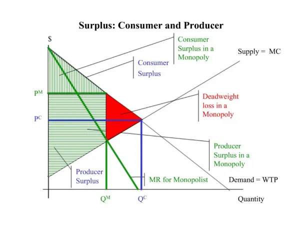
Consumer Surplus and Welfare We saw earlier that, following a price change,
Consumer Surplus and Welfare p1 a b Marshallian Demand x1
Summary • Indifference curves • Marginal rates of substitution • Marshallian demand functions • Types of goods • Indirect utility function • Consumer surplus and welfare • Roy’s Identity
Readings • Texts: • Varian, Intermediate Economics (7th ed.) chapters 4, 5, 6, 14. • Varian, Microeconomic Analysis, chapter 7