Download
1 / 15
150 likes | 264 Vues
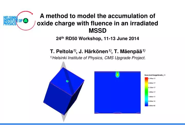
A method to model the accumulation of oxide charge with fluence in an irradiated MSSD 24 th RD50 Workshop, 11-13 June 2014. T. Peltola 1) , J. Härkönen 1) , T. Mäenpää 1) 1) Helsinki Institute of Physics, CMS Upgrade Project. Outline Motivation & method to determine CCE(x)

E N D
A method to model the accumulation of oxide charge with fluence in an irradiated MSSD • 24th RD50 Workshop, 11-13 June 2014 • T. Peltola1), J. Härkönen1), T. Mäenpää1) • 1)Helsinki Institute of Physics, CMS Upgrade Project.
Outline • Motivation & method to determine CCE(x) • Motivation: why non-uniform 3-level defect model? • CCE(x): Iteration method • CCE(x): proton model vsnon-unif. 3-l model • Qf(Φ) & c(Φ) modelling • Measured CCE(x) vs simulation: • d & η varied • d = constant • Qf(Φ) & c(Φ) of region 5 200P MSSD Timo Peltola, 24th RD50 Workshop, 11-13 June 2014
Motivation & method to determine CCE(x) Timo Peltola, 24th RD50 Workshop, 11-13 June 2014
Non-unif. 3-level defect model: Motivation • 3-level model within 2 μm of device surface + proton model in the bulk: • Rint (fig. 1) & Cint (fig. 2) in line with measurement also at high fluence & Qf • Non-unif. 3-l model can be tuned to equal bulk properties (TCT, Vfd & Ileak) with proton model → suitable tool to investigate CCE(x) Figure 1: Rint SiBT measured CCE(x) for proton & mixed fluences (T. Mäenpää): Φeq=1.4e15 cm-2 Center of strip Figure 2: Cint • Non-unif. 3-l model: n-on-p, r5 • @ F=1.5e15 cm-2 Φeq=3e14 cm-2 Center of gap • f = 1 MHz FZ200Y, region 5 MCz200P, region 5 Timo Peltola, 24th RD50 Workshop, 11-13 June 2014
CCE(x) @ Φeq= 1.5e15 cm-2: Iteration method • CCE loss: • 60 μm • 0 μm • 40.6% • Qf increases • → Qcoll decreases • Qf increases • → Qcoll increases 2nd strip center strip • 37.3% • 31.1% mip positions • 25.4% • 20.3% • 17.5% • Principle of CCE(x) simulation for given c(shallow acc.) & voltage • 5 strip 200P, region 5 @ Φeq=1.5e15 cm-2, V=-1 kV, T=253 K • Acceptor traps remove both inversion layer & signal electrons: better radiation damage induced strip isolation → larger CCE loss between the strips • Increased Qf fills more traps → CCE loss decreases, undepleted region between strips grows • Space charge dominated region • Oxide charge dominated region Timo Peltola, 24th RD50 Workshop, 11-13 June 2014
CCE(x): proton model vs non-unif. 3-l model 200P region 5 @ Φeq=1.5e15 cm-2, V=-1 kV, T=253 K • Proton model (tuned by R. Eber) Proton model • Qf= 1.2e12 cm-2: CCE loss ≈ 15 % • Qf~ 1.5e12 cm-2: no strip isolation & cluster CCE ~0.5 of expected due to undepleted region produced by highQf • 3-level model within 2 μm of device surface • Qf= 1.2e12 cm-2: CCE loss ≈ 41 % • Qf= 2e12 cm-2: increased charge sharing when mip position ≥ 30 μm from center strip, but still producing position information • When strips are isolated both models produce same cluster CCE at the center of the strip Non-unif. 3-l model Center of gap = 60 μm Center of strip = 0 Timo Peltola, 24th RD50 Workshop, 11-13 June 2014
proton model vs non-unif. 3-l model: electron density • Electron density @ Qf= 1.2e12 cm-2, V=-1 kV from previous slide • Effect of acceptor traps in non-unif. 3-l model is clearly visible: • ~5 orders of magnitude difference between models (from n+ to p-stop) • Cut @ 50 nm below oxide n+ n+ p-stops 2nd strip center strip Timo Peltola, 24th RD50 Workshop, 11-13 June 2014
Qf(Φ) & c(Φ) modelling Timo Peltola, 24th RD50 Workshop, 11-13 June 2014
Measured CCE(x) vs simulation: d & η varied • 200P Region 5: p+ Φeq=3e14 cm-2, V=-990 V, T=253 K • SiBT measured CCE loss(FZ200P/Y, MCz200P) @ V=600 – 990 V: 26.5±1.1% • Double p-stop: dp=1.5 μm=dimplant, wp=4 μm,spacing=6 μm • Approach: • Iterate η to find CCE loss within measured error margins @ Qf~5e11 cm-2 • Change 3-level model thickness to preserve transient signal shape • 3.1% • Charge multiplication region • 8.5% • Oxide charge dominated region • Cut @ implant curvature • E(x) between 2nd & center strip for η=40 cm-1, Np=1e16 cm-3 • Two low CCE loss regions observed in Qf scan • Not seen in Φeq=1.5e15 cm-2 CCE loss simulations, because of higher Qf values (1.2e12…2e12 cm-2) • Interpretation: At very low Qf high E produces charge multiplication → additional charge carriers fill traps → CCE loss decreases significantly → New approach: keep 3-level region thickness constant & add constant factor to shallow level c Timo Peltola, 24th RD50 Workshop, 11-13 June 2014
Measured CCE(x) vs simulation: d = constant • 3-level region: d=2 µm, strip length = 3.049 cm • Φeq≈1.5e15 cm-2 has largest statistics at ~600 V → simulation V adjusted • Target Qf~5e11 and ~1.5e12 cm-2 for given fluences • Measurement: 6 μm resolution • Measured CCE loss(FZ200P/Y, MCz200P) @ • Φeq (p+) = 3e14 cm-2, V = 600 – 990 V: 26.5 ± 1.1 % • Measured CCE loss(FZ200P/Y, MCz200P/Y) @ • Φeq (mixed) = (1.4 ± 0.1)e15 cm-2, V = 606 ± 2 V: 30 ± 2 % Φeq=3e14 cm-2 V=-990 V Qf=(1.405–1.425)e12 cm-2 Qf=(4.6–6.0)e11 cm-2 Φeq =1.5e15 cm-2 V=-608 V Timo Peltola, 24th RD50 Workshop, 11-13 June 2014
Qf(Φ) & c(Φ) in p+ irradiated region 5 200P • Qf of non-irradiated 200P from measured initial dip of Cint, that is reproduced by decreasing Qf=2.7e10cm-2 • c(shallow acc.) parametrized by using ‘fixed’ values of Qf → fixed c, parametrizedQf • Increase of the shallow acceptor concentration is found to be ~0.5 ofconstant factor at the given fluence range • Qf = 5e10 cm-2 • Qf = 2.7e10 cm-2 Cint(V) Cint(V) Timo Peltola, 24th RD50 Workshop, 11-13 June 2014
Summary • When position dependency of CCE is modeled by non-unif. 3-l defect model, it is governed by Qf and shallow acceptor concentration • By tuning these two parameters it is possible to reproduce measured CCE loss between strips for given fluence • If one of the parameters is fixed, the other can be solved reliably→ potential for Qf(Φ) parametrization • With test values of Qf the shallow acceptor concentration does not have strong dependence on fluence in the range 3e14 → 1.5e15 cm-2 Timo Peltola, 24th RD50 Workshop, 11-13 June 2014
Backup: SiBT measured CCE loss between strips Signal loss in-between strips (p=120µm, w/p~0.23) non-irradiated FTH200Y MCz200N FTH200P FTH200N No loss before irrad.; after irrad. ~30% loss; all technologies similar [Phase-2 Outer TK Sensors Review] MCz200N MCz200P MCz200Y FZ200N mixed irradiated 1.5e15neq/cm² Timo Peltola, 24th RD50 Workshop, 11-13 June 2014
Backup: Measured Rint 109 P and Y types:Rint P and Y types:Rint • Measurement (W. Treberspurg) • DC-CAP F=5e14 cm-2 F=1e15 cm-2 106 Timo Peltola, 24th RD50 Workshop, 11-13 June 2014
Backup: simulated Rint& Cint • 3 strip structure, Vstrip1 = Vstrip3 = 0, Vstrip2 = LV and 0 V • V = -HV at the backplane • Interstip resistance (Rint) is defined as (Induced Current Method): • Rint is plotted as a function of appliedvoltageV • Cint simulation principle • Electrical circuit diagram of Rint measurement : Cint = 2*[AC(1,2)+DC(1,2)+AC(1)DC(2)+DC(1)AC(2)] • Rint simulation principle • Vstrip1 = 0 1: Vstrip2 = LV 2: Vstrip2 = 0 • Vstrip3 = 0 Timo Peltola, 24th RD50 Workshop, 11-13 June 2014