Download
1 / 7
70 likes | 79 Vues
11. Spectral Lines II. Rutten: 5.1, 5.2 Line formation Eddington-Milne Curve of Growth. Curve of Growth. Curve of Growth is a theoretical plot of line equivalent width against line optical depth, usually plotted as log( W l ) – log( t ).

E N D
11. Spectral Lines II • Rutten: 5.1, 5.2 • Line formation • Eddington-Milne • Curve of Growth
Curve of Growth Curve of Growth is a theoretical plot of line equivalent width against line optical depth, usually plotted as log(Wl) – log(t). The Wl – t relation is seen in the Schuster-Schwarzschild model atmosphere: continuous spectrum is emitted from a deep layer, Ic = Bl(TR), second reversing layer at TL absorbs the spectral lines. Radiation we observe is (from L2): where tl is the optical depth of the reversing layer given by: where Ni is the column density along LOS (m-2) of particles in lower level i.
The relative line depression is: Where Dmax = [Bl(TR) - Bl(TL)] / Bl(TR) the maximum depression for very strong lines. The equivalent width is showing how Wl relates to t and hence also Ni and f. The curve of growth can be split into three regimes depending on the optical depth (line strength): weak, saturated, and strong lines.
1. Weak Lines: For tl << 1, exp(- tl) ~ 1 – tl, so D ~ Dmaxtl. The Voigt profile is approximated by Doppler because opacity is too small to map damping wings into emergent spectrum. Replacing H(a,v) with exp(-[Dl/DlD]2) with area p½DlD gives: Wl ~ fNi. Part 1 of curve of growth is Doppler part and has slope 1:1. Linear increase due to optical thinness of reversing layer. 2. Saturated Lines: For tl > 1, line cannot be deeper than Dmax. The line width increases with tl0 and Where Q ~ 2 – 4. This is part 2 of curve of growth or the shoulder.
3. Strong Lines: For tl >> 1, the core doesn’t change any more. Line centre is fixed at Dmax, but line wings have tl < 1 and may grow in optically thin fashion to increase Wl. For large tl0 the wings contribute a lot because they map the damping part of A drop off with Dl that is less steep than the exponential decay of the Doppler core. In the damping part of H(a,v) we write: which gives: Thus part 3 or the damping part scales as Wl ~ (atl0)½ ~ (fNig)½ .
log Wl 3 1 2 2 1 1 1 log tl0 Ic(TR) 0 1 2 3 Dl Il Bl(TL) Dmax 0 1 l0
Classical Curve of Growth Fitting The strategy is to analyze lines via a curve of growth to determine abundances, damping parameter a, excitation temperature Texc, and microturbulence xmicro. Plot measured Wls as log(Wl/l) against where… Changing parameters changes the shape of theoretical curve of growth. By minimizing scatter of data can derive physical parameters.