Download
1 / 21
220 likes | 265 Vues
POPULATION VS. SAMPLE. Population: a collection of ALL outcomes, responses, measurements or counts that are of interest. Sample: a subset of a population What are some examples of population? Ex: BHS What are some examples of samples? Ex: Sample of BHS could be the Senior Class.

E N D
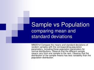
POPULATION VS. SAMPLE Population:a collection of ALL outcomes, responses, measurements or counts that are of interest. Sample:a subset of a population What are some examples of population? Ex: BHS What are some examples of samples? Ex: Sample of BHS could be the Senior Class
INTERPRETING HISTOGRAMS • Look at OVERALL PATTERN • Center • Spread • Shape • Symmetric? • Skewed Right (tail right)? • Skewed Left (tail left)? • Unimodal, bimodal, multimodal? • Look at striking DEVIATIONS • Called OUTLIERS(lies outside the overall pattern)
PANCAKES VS. SKYSCRAPERS • Histograms with too few intervals Skyscrapers Histograms with too many intervals Pancakes
HISTOGRAM ON CALCULATOR Stat, 1 (to enter data) Stat plot (to choose histogram) Zoom 9 (to set up axis) Window (to modify widths of bars)
WHY USE A STEMPLOT? Details: • If data has too many digits, you can round off: • 4.1385 4.14 • 5.2273 5.23 • If data falls into too few stems, you can split them up, 0-4 and 5-9 so each stem appears twice. Babe Ruth Home Runs becomes: 2 2 2 5 3 4 3 5 4 11 4 66679 5 44 5 9 6 0 key 7 2 = 72 Easier to find the middle Shows the shape of the distribution
Median is a resistant measure of center • When are the mean and median the same? • When are they different? • Is the mean or median enough? • Only gives information about the center. • We want to know about spread and variability • Range – includes outliers • So, it is often best to look at the middle two quartiles (the middle half of the data)
Quartiles, divides data into 4 equal parts: 1. Arrange data in order and locate the median (also Q2) 2. The first quartile, Q1, is the median of the first half of the data 3. The third quartile, Q3, is the median of the second half of the data Example: 5, 7, 10, 14, 18 19, 25, 29, 31, 33 Q1 = 10 Q2 = 18.5 Q3 = 29 Note: If odd number of data, do not include the median in your Q1 and Q3 Babe Ruth Data: 22, 25, 34, 35, 41, 41, 46, 46, 46, 47, 49, 54, 54, 59, 60 | | | Q1 = 35 Q2 = 46 Q3 = 54 Interquartile Range (IQR) = Q3 - Q1 = 54-35 = 19
One rule of thumb to identify outliers is to compute 1.5 * IQR. If a value falls • above Q3 + 1.5 * IQR or • below Q1 - 1.5 * IQR, then the value is an outlier.
For example, with Babe Ruth the IQR = 19. So what is an outlier? 1.5*19 = 28.5 54 + 28.5 = 82.5 and 35 – 28.5 = 6.5 So, there are no outliers
FIVE NUMBER SUMMARY Here is an example: A Swiss study looked at the # of hysterectomies performed by 15 male doctors: 20 25 25 27 28 31 33 34 36 37 44 50 59 85 86 Find the 5 number summary for this data set. • A convenient way to describe the center and spread of a data set is the five number summary. • The five number summary is defined as: Min (value), Q1, Median, Q3, Max(value)
** Must have a scale below the box plot – make the scale first, then plot the five number summary. Min Q1 Med Q3 Max 20 27 34 50 86 Here is a box plotof this data. A very powerful graph
CALCULATOR INSTRUCTIONS • BOXPLOT • Enter data into list • Stat plot • Use down arrows to select the box plot and press ENTER • Press ZOOM • Press down arrow to ZoomStat and press ENTER • 5 NUMBER SUMMARY • Press STAT • Press the right arrow to display the choices for STAT CALC • Press ENTER to choose 1-Var Stats
ANOTHER MEASURE OF SPREAD:STANDARD DEVIATION • A measure of spread that we have discussed is the 5 number summary. We use that when using the median as measure of center. • A measure of spread used when using the mean as measure of center is called standard deviation. Measure of CenterMeasure of Spread Median 5 number summary Mean standard deviation
CALCULATION OF STANDARD DEVIATION 1. Find the mean. 2. Find the difference between each data item and the mean. Distance from the mean. 3. Square each difference and add them. Gets rid of any negatives and makes the larger differences even larger. 4. Find the average (mean) of these squared differences, but need to divide by n-1 rather than n. Average squared distance from the mean. 5. Take the square root of this average. Just average distance from the mean.
HERE IS HOW TO COMPUTE THE STANDARD DEVIATION.DATA: SET 12, 13, 13, 27, 27, 28. WHAT IS THE MEAN? 20 12-20 = -8 64 49 13-20 = -7 13-20 = -7 49 49 27-20 = 7 27-20 = 7 49 28-20 = 8 64 Add all the (xi-mean)2 and divide by n-1 and take the square root. 64+49+49+49+49+64= 324/(6-1)=64.8. (64.8)=8.05
The standard deviation (s) is the square root of the variance. • The variance (s2) is the average of the squares of the differences of each observation from the mean. • Here is the formula for standard deviation: Where xi = each data point xbar = sample mean n = number of values
WHY N-1? • Theof the deviations, no squares, is always 0. So once we know n-1 of the deviations the nth one is known also.We are not averaging n unrelated numbers. The idea of variance is the average squares of the deviations of observations from the mean. So why do we average by dividing by n-1 instead of n?
SO… • The numbers are related. • Only n-1 of the squared deviations can vary freely so we average by dividing by n-1. n-1 is called the degrees of freedom. • Ex: If you have 4 markers and 4 people to choose their markers, how many of them will have FREEDOM of choice?
Probability Histogram Cumulative Histogram
ALWAYS PLOT DATA FIRST!