Download
1 / 23
230 likes | 401 Vues
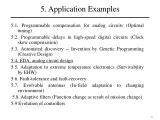
5. Application Examples. 5.1. Programmable compensation for analog circuits (Optimal tuning) 5.2. Programmable delays in high-speed digital circuits (Clock skew compensation) 5.3. Automated discovery – Invention by Genetic Programming (Creative Design) 5.4. EDA Tools, analog circuit design

E N D
5. Application Examples 5.1. Programmable compensation for analog circuits (Optimal tuning) 5.2. Programmable delays in high-speed digital circuits (Clock skew compensation) 5.3. Automated discovery – Invention by Genetic Programming (Creative Design) 5.4. EDA Tools, analog circuit design 5.5. Adaptation to extreme temperature electronics (Survivability by EHW) 5.6. Fault-tolerance and fault-recovery 5.7. Evolvable antennas (In-field adaptation to changing environment) 5.8. Adaptive filters (Function change as result of mission change) 5.9 Evolution of controllers 1
Hardware Evolution of Analog Speed Controllers for a DC Motor • Development of an autonomous, self-configurable controller for use on a remotely located platform • Adaptation of controller to environmental changes that would otherwise degrade performance • Temperature extremes • Ionizing radiation • Variation in the controlled dynamic system • Reconfiguration of controller structure • Use of degraded components: electronic and mechanical • Exclusion of failed components: sensor failures • Response to changing mission requirements • Applicable to platforms for exploration of space or extreme terrestrial environments Work by Gwaltney (MSFC) and Ferguson (JPL) 2
Motivation for This Work • Motor driven systems are ubiquitous in commercial, industrial, military and aerospace applications • By-wire technology relies extensively on electromechanical actuators • Aircraft, fly-by-wire • Automobiles, drive-by-wire • Recent space transportation vehicle concepts • Availability of programmable analog or mixed-signal devices makes the implementation of analog control loops attractive at the actuator and subsystem level • Can be as easily modified as software 3
Approach Use of JPL developed Stand Alone Board Level Evolvable (SABLE) System as platform for controller evolution • Employs the JPL second generation Field Programmable Transistor Array (FPTA2) • GA implemented in firmware and executed on a Digital Signal Processor (DSP) single board computer (SBC) • FPTA2 configuration through digital interface on SBC • 16 bit DAC provides stimulus of the FPTA2 • 16-bit , multi-channel ADC module captures FPTA2 output and other analog signals for fitness evaluation 4
SABLES 5
JPL FPTA2 Cell Layout 0 3 12 15 48 51 60 63 1 2 13 14 49 50 61 62 O(64) 8 11 52 55 56 59 4 7 10 53 54 57 58 5 6 9 16 19 28 31 32 35 44 47 17 18 29 30 33 34 45 46 20 23 24 27 36 39 40 43 21 22 25 26 37 38 41 42 N W E I(96) S 96 analog inputs 64 analog outputs Interconnection between cells • New technology: TSMC 0.18 – 1.8v; • 64 reconfigurable cells; 6
Evolvable Controller Configuration DSP w/Analog Module DC Motor Tachometer Current Control Motor Driver CMD FPTA2 Error = CMD - Feedback Diagram of the experimental configuration for hardware evolution of analog motor speed controllers 8
Evolvable Controller Configuration Second motor operated as a generator and used to provide load 9
Baseline Analog Controller Design Most widely used form of analog controller is the Proportional-Integral (PI) Controller • Used for motor current control and speed control PI control law is represented by Where e(t) is error between desired plant response and measured plant response, KP is proportional gain, KI is integral gain or time constant, KD is derivative gain 10
Baseline Analog PI Controller _ _ _ 1.1K 20K 20K Vtach 1.8V + + + _ 1.1K Ve + 20K Pot 1.1K 20K Vcmd 1.1K 20K Vbias2 (0 – 1.8V) R2 C 1.8V R1 Vu 10K, 1% Vbias1 (0.9V) 10K, 1% PI Controller for 1.8V supply and 1.8V unipolar signal range Vu = (Ve - Vbias2)(R2/R1 + 1/R1Cs) + Ve Ve = Vcmd/2 +0.9 – Vtach/2 R1 = 10K, R2 =200K, C=0.47uF, Vbias2 = 0.865 Vcmd and Vtach, Ve and Vu are 0 – 1.8V signals 11
Response Using PI Controller Response with no offset between command and tachometer feedback is achieved by adjusting Vbias2 Motor speed response obtained using PI controller. Vsp is gray, Vtach is black 12
Evolution of Analog Controllers • Two FPTA cells used • Cell 1 provided with motor speed command and tachometer feedback. Responsible for producing current command to motor driver. • Cell 0 used to provide support electronics for cell 1 • Evolutionary Algorithm • Standard GA • Population initially seeded with randomly generated FPTA2 configurations • Population constrained to force the cell 1 switches closed that connect the speed command and tachometer feedback to the cell • All closed-loop controllers must use a command and feedback to produce an error signal • DAC module generates sinusoid for motor speed command • ADC module simultaneously records command and feedback signals for fitness evaluation 13
Evolution of Analog Controllers Case 1 Case 2 • Many Controllers were evolved using varying fitness functions and conditions • Experimental results for two evolved controllers will be presented. The fitness functions and conditions for the evolution of the two cases given differ as shown below • Penalty for not connecting speed command or feedback signal to cell 1 • 100 individuals in the population • 2 Hz sinusoid for speed command • Forced closure of switches connecting speed command and feedback signal to cell 1 • 200 individuals in the population • 3 Hz sinusoid for speed command 14
Experimental Results Case 2 Evolved Controller Case 1 Evolved Controller Motor speed response obtained using evolved controllers. Vsp is gray, Vtach is black 15
Experimental Results The Case 1 response is compared to the baseline response obtained using the PI controller in the tables below • The increase in mean error indicates higher constant offset error in the response. In PI controller this offset is removed via adjustment of Vbias2. FPTA is given no such bias input. • Experiments show the cell 0 is providing a biasing action for cell 1 16
Experimental Results Case 2 is interesting in that the switches (S54, S61, S62, S63) that route the tachometer feedback to the interior of the reconfigurable cell are all open. • Removal of the feedback signal causes the controller to malfunction • This implies an unanticipated pathway exists in the cell that is being exploited by the evolution • This is the only example obtained to date that uses this exploit. 17
JPL FPTA2 Cell Schematic Tach Feedback Speed Command In Case 2, Switches 54, 61, 62 and 63 are open in Cell 1 18
Experimental Results • The evolved controllers are providing a good response using two adjacent cells in the FPTA to perform a similar function to four op-amps, a collection of 12 resistors and one capacitor. • The FPTA switches have inherent resistance on the order of KOhms • Each cell has 14 transistors to be used as functional components • Cells can be used to implement op-amps by using external passive components and bias voltages • No external components or bias provided • The capability of the controller to respond to inputs of varying amplitude and frequency and varying load are presented on subsequent slides 19
Response to Speed Command Changes Case 1 Evolved Controller 20 Channel 1 is command, Ch2 is feedback, Ch3 is controller output, Ch4 is motor current and ChM is the error between Ch1 and Ch2
Response to Load Changes Case 1 Evolved Controller No Load Full Load Note the changes in controller output (ch3) and current (Ch4). In the No load case, the positive current oscillates , but is steady in the full load case. Oscillation is sort of a PWM action. So steady current indicates higher torque in response to higher load. Negative current magnitude increases in Full Load Plot 21
Response to Load Changes Case 1 Evolved Controller No Load Full Load Note the changes in controller output (ch3) and current (Ch4). In the No load case, the positive current oscillates , but is steady in the full load case. Oscillation is sort of a PWM action. So steady current indicates higher torque in response to higher load. Negative current magnitude increases in Full Load Plot 22
Summary • The results presented show the FPTA2 can be used to evolve simple analog closed-loop controllers that provide good response in comparison with a PI controller • Evolved design uses less transistors than the conventional design, and no external components. • Neglecting programmable overhead, considering functional components only • Relatively slow response of many practical servomotor-driven systems is a time bottleneck that increases time to convergence • Can be addressed through novel controller configurations and approach to evolution 23