Review of basic statistics

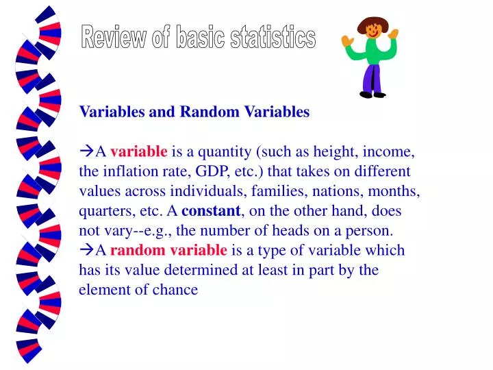
1. Review of basic statistics • Variables and Random Variables • A variable is a quantity (such as height, income, the inflation rate, GDP, etc.) that takes on different values across individuals, families, nations, months, quarters, etc. A constant, on the other hand, does not vary--e.g., the number of heads on a person. • A random variable is a type of variable which has its value determined at least in part by the element of chance

2. Measures of Central Tendency • The mode, median, and mean are measures of the central tendency of a random variable such as the height of males. If the statement is made with respect to this variable that “the mode is 5'10",” it means that most common height (or the height which occurs with the greatest frequency) among males is 5'10". • Themedian is the value of the random variable such that half the observations are above it and half below it. To say that “median family income in the U.S. is $38,450" is to say that half of U.S. households have an income below that figure and half above it.

3. The populationmean (symbolized by the Greek letter µ) is the average value of the variable for the population. Let m denote the number of observations (corresponding to the size of the population). Thus, we have: • Suppose we want to know the average height of adult males in the U.S. The practical approach would be to measure a representative sample (meaning, for example, that basketball players would not be disproportionately represented in the sample) of the population rather than the entire population. That is, we estimate the population mean by calculating a sample mean( ). Let n be the number of observations in our sample. Thus we have:

4. Measures of Dispersion • Often we are interested in looking at the degree of dispersion of a random variable about its mean value. That is, are our observations of adult male height all bunched up around the mean or do we have wide dispersion about the mean? The population variance (2) is a measure of the dispersion of a random variable . The variance of random variable X is defined as:

5. If we observe only a representative sample of the population, then : (1) µ is unknown; and (2) all the Xi ’ s are not known. Thus, we estimate 2 by substituting  for µ and summing across our sample observations of X This is called a sample variance (s2): • Note that we must divide through by n - 1 to obtain an unbaised estimate of2 --that is s2 is an unbaised estimator of 2 if E(s2 ) = 2 • The population standard deviation () is given by the square root of the population variance ( 2). You can think of as the “average deviation from the mean.” In the case of male adult height, one would like to see that measure expressed in inches--hence we take the square root of the variance. • Similarly, the sample standard deviation (s) is given by the square root of the sample variance (s2).

6. Probability Distributions • The probability density function of variable X is constructed such that, for any interval (a, b), the probability that X takes on a value in that interval is the total area under the curve between a and b. Expressed in terms of integral calculus, we have:

7. You should be familiar with this diagram P(X) Area under curve represents probability a b X

8. The standard normal distribution • The normal distribution is probability density function which is symmetric about the mean--i.e., the left-hand side of the distribution is a mirror image of the right-hand side. The formula for the normal probability density function is given by:

9. The normal distribution 68.27% 95.45%  -2 -   2

10. A random variable Z is said to be standard normal if it is normally distributed with mean of zero or and a variance of 1. If X is normally distributed with mean µ and variance 2, we abbreviate with the expression: • X ~ N(, 2) • Thus, the expression used to indicate that the distribution of Z is standard normal is: • Z ~ N(0, 1)

11. The standard normal distribution • For example: • If a = 1.93, then Pr(Z  a ) = 0.1093 • And Pr(Z  a ) 1 - 0.1093 = 0.8907 P(Z) 0 a Pr(Z > a) when Z ~ N(0, 1)

12. Correlation of Random Variables • To say that random variables X and Y are correlated is to say that changes in X are associated with changes in Y in the probabilistic or statistical sense. However, this does not necessarily mean that a change in X was the cause of a change in Y, or vice-versa. That is, “correlation does not imply causality.” • Technically speaking, the statement “X and Y are positively correlated” means that the covariance between random variables X and Y is positive (or greater than zero).

13. 1, X > E(X) and Y > E(Y) 2, X < E(X) and Y > E(Y) 3, X < E(X) and Y < E(Y) 4, X > E(X) and Y < E(Y) Y 2 1 E(Y) 3 4 0 E(X) X X and Y are positively correlated random variables

14. The sample covariance between X and Y (i.e., our estimate of the covariance when we do not observe the entire populations of X’s or Y’s) is given by the following formula (the “hat” indicates an estimate): • The covariance is positive if above average values of X tend to be paired with above average values of Y, and vice versa. The covariance is negative (and hence the variables are negatively correlated) if below average values of X tend to be paired with above average values of Y, and vice-versa. The magnitude of the covariance depends partly on the unit of measurement. Hence, we cannot depend on the size of the covariance to give an accurate measure of the strength of the relationship

15. The correlation coefficient ( ) is a unit-free measure of correlation. The sample correlation coefficient is given by: • It will always be the case that: -1   1. • If  = 1, there is a perfect positive ( linear) correlation between X and Y. If  = -1, there is a perfect negative (linear) correlate between X and Y.