Download
1 / 32
330 likes | 407 Vues
Equilibrium Finite Elements. University of Sheffield, 7 th September 2009 Angus Ramsay & Edward Maunder. Introduction. Who are we? Partners in RMA Fellows of University of Exeter What is our aim? Safe structural analysis and design optimisation How do we realise our aims?

E N D
Equilibrium Finite Elements University of Sheffield, 7th September 2009 Angus Ramsay & Edward Maunder
Introduction • Who are we? • Partners in RMA • Fellows of University of Exeter • What is our aim? • Safe structural analysis and design optimisation • How do we realise our aims? • EFE an Equilibrium Finite Element system
Contents • Displacement versus Equilibrium Formulation • Theoretical • Practical • EFE the Software • Features of the software • Live demonstration of software • Design Optimisation - a Bespoke Application • Recent Research at RMA • Plates – upper/lower bound limit analysis
A Time Line for Equilibrium Elements RMA & EFE Ramsay Maunder Turner et al Constant strain triangle 1950 1960 1970 1980 1990 2000 2010 Heyman Master Safe Theorem Robinson Equilibrium Models Teixeira de Freitas & Moitinho de Almeida Hybrid Formulation Fraeijs de Veubeke Equilibrium Formulation
Displacement versus Equilibrium Elements Hybrid equilibrium element Conventional Displacement element Semi-continuous statically admissible stress fields = S s Discontinuous side displacements = V v
Modelling with Equilibrium Elements • Sufficient elements to model geometry • hp-refinement – local and/or global • Point displacements/forces inadmissible • Modelled (more realistically) as line or patch loads
Discontinuous Edge Displacements p=2 p=1 p=0, 4 elements 2500 elements 100 elements
Strong Equilibrium Error in Point Displacement EFE 1.13% Abaqus (linear) 10.73% Abaqus (quadratic) 1.70%
Heyman Sleipner Collapse (1991) Computer Aided Catastrophe
Presentation of Results (Basic) Equilibrating boundary tractions Equilibrating model sectioning
Presentation of Results (Advanced) Stress trajectories Thrust lines
EFE the software (a vehicle for exploiting equilibrium elements) • Geometry based modelling • Properties, loads etc applied to geometry rather than mesh • Direct access to quantities of engineering interest • Numerical and graphical • Real-Time Analysis Capabilities • Changes to model parameters immediately prompts re-analysis and presentation of results • Design Optimisation Features • Model parameters form variables, structural response forms objectives and constraints
Program Characteristics • Written in Compaq Visual Fortran (F90 + IMSL) • the engineers programming language • Number of subroutines/functions > 4000 • each routine approx single A4 page – verbose style • Number of calls per subroutine > 3 • non-linear, good utilisation, potential for future development • Number of dialogs > 300 • user-friendly • Basic graphics (not OpenGL or similar – yet!) • adequate for current demands
Landing Slab • Analyses • elastic analysis • upper-bound limit analysis • Demonstrate • real-time capabilities • post-processing features • geometric optimisation Equal isotropic reinforcement top and bottom Simply Supported along three edges Corner column UDL
Axial Turbine Disc • Analyses • elastic analysis Axis of rotation Axis of symmetry Angular velocity Blade Load Geometric master variable Geometric slave variables • Demonstrate • geometric variables • design optimisation Objective – minimise mass Constraint – burst speed margin
Bespoke Applications Geometry: Disc outer radius = 0.05m Disc axial extent = 0.005m Loading: Speed = 41,000 rev/min Number of blades = 21 Mass per blade = 1.03g Blade radius = .052m Material = Aluminium Alloy Results: Burst margin = 1.41 Fatigue life = 20,000 start-stop cycles
Limit Analyses for Flat Slabs • Flat slabs – assessment of ULS • Johansen’s yield line & Hillerborg’s strip methods • Limit analyses exploiting equilibrium models & finite elements • Application to a typical flat slab and its column zones • Future developments
Heyman Pipers Row car park collapsed 4th floor slab - 1997
EFE: Equilibrium Finite Elements • Morley constant moment element to hybrid equilibrium elements of general degree Morley general hybrid
Reinforced Concrete Flat Slab RC flat slab – plan geometrical model in EFE designed by McAleer & Rushe Group with zones of reinforcement
Moments and Shears principal moments principal moment vectors of a linear elastic reference solution: statically admissible – elements of degree 4 principal shears
Elastic Analysis elastic deflections Transverse shear Bending moments
Yield-Line Analysis basic mechanism based on rigid Morley elements contour lines of a collapse mechanism yield lines of a collapse mechanism
Equilibrium from Yield Line Solution principal moment vectors recovered in Morley elements (an un-optimised “lower bound” solution)
Mxy Myy Mxx Quadratic constraints & a Linearisation biconic yield surface for orthotropic reinforcement
Hyperstatic Variables closed star patch of elements formation of hyperstatic moment fields
Moment redistribution in a column zone moments direct from yield line analysis: upper bound = 27.05, “lower bound” = 9.22 optimised redistribution of moments based on biconic yield surfaces: 21.99
Future developments for lower bounds • Refine the equilibrium elements for lower bound optimisation, include shear forces • Initiate lower bound optimisation from an equilibrated linear elastic reference solution & incorporate EC2 constraints e.g. 30% moment redistribution • Use NLP to exploit the quadratic nature of the yield constraints for moments • Extend the basis of hyperstatic moment fields • Incorporate shear into yield criteria • Incorporate flexible columns and membrane forces