Download
1 / 21
210 likes | 323 Vues
Chapter Two: Summarizing and Graphing Data. 2.2: Frequency Distributions 2.3: ** Histograms **. Summarizing Data. Human beings cannot interpret large amounts of raw data. Here are State Unemployment Rates (July 2012) from BLS:. Summarizing Data.

E N D
Chapter Two:Summarizing and Graphing Data 2.2: Frequency Distributions 2.3: ** Histograms **
Summarizing Data • Human beings cannot interpret large amounts of raw data. Here are State Unemployment Rates (July 2012) from BLS:
Summarizing Data • It is crucial to organize, summarize, and display data in a way that… • …accurately reflects the overall characteristics of the data. • …does not overstate or underemphasize patterns or trends in the data. • …is easy for human beings to interpret. • …is useful for later statistical analysis.
Summarizing Data We will consider the following general features: • Center: A “typical” or “average” value that represents the “middle” or the data. • Variation: A measure of how data values change or vary for different individuals. • Distribution: The overall pattern or “shape” of the data. (symmetric, skewed, “bell curve,” etc.) • Outliers: Individual values that are “unusual” compared to the majority of the data set.
Quantitative vs. Categorical Data Quantitative data consist of number that represent counts or measurements. All quantitative data is numerical, but not all numerical data is quantitative. Data with a unit of measurement (seconds, feet, pounds, dollars, etc.) is quantitative. Numerical data used as a label or range of values (Student ID Number, 20-25 years) is not quantitative.
Examples: Quantitative Data The University keeps the following quantitative data about each student. Grade Point Average Number of Credit Hours Completed Age Amount of money owed for tuition Other examples?
Categorical Data Data that are not quantitative are called categorical. Non-numerical data must be categorical. Numerical data that serves to label or identify individuals are categorical (Example: Social Security Number). A useful guide: Would it make sense to consider an average value? If not, treat the data as categorical.
Examples: Categorical Data The University keeps the following categorical data about each student: Name Laker ID Number Date of Birth Gender Residency (“in-state” or “out-of-state”) Other?
Frequency Distributions • Instead of displaying a list of data values for all individual, we can summarize as follows: • Group the values into several categories (or classes) such that each individual belongs to exactly one category. • For each category, give the number of individuals with values in that category. This number is called the frequency of the category. • Example: Rather than listing each student’s Gender, we can summarize as follows: Female: ____ Male: ____
Example: State Unemployment For quantitative data (must be numerical), we often group nearby values together. Here is the July 2012 state unemployment data:
Relative Frequency Table Alternatively, we can express the frequency for each category as a percentage of the number of values in the data set:
Cumulative Frequencies Less common is the cumulative frequency (or percent), where we count the number/percent of individual less than a certain value:
Histograms Section 2.3
** Histograms ** • A histogram is a graphical representation of a frequency table. Here is the state unemployment data from earlier: Number of states Percent Unemployed
** Histograms ** Here is the same data, using smaller (more narrow) classes: Number of states Percent Unemployed
Making Histograms • The histograms in today’s slides were generated using the JMP software package. The numbers above each bar are there for your convenience (these do not appear in the textbook). • You should not worry about making histograms (or even frequency tables) by hand. Software will do this for you! • You should focus on how to read and interpret a histogram. This is a crucial skill!
Example: Exam 1 Scores Count Exam Score • The histogram above shows the scores on Exam 1 from a previous semester of this course. • JMP includes the left endpoint in each interval, but not the right endpoint. Classes are 10-19, 20-29, etc. • What does this tell you about scores on Exam 1? 17
Interpreting Histograms Some questions about the Exam 1 scores: • How many students scored 80 or better? • How many students scored less than 60? • How many students scored in the 60-79 range? • Does the histogram show any “unusual” scores? • How many students scored 75 or better?
Normal Distributions • In many cases, we have a histogram with that has the following features: • Approximate “bell” shape. • Strong (not always perfect) left/right symmetry • A single “peak” in the middle, short “tails” on the left and right sides. • The State Unemployment data had these features. The Exam 1 data did not.
Example: Approximately Normal • State unemployment data, with the approximating “bell” in red: Number of states Percent Unemployed
Normal Distributions • “Normal” refers to a very specific type of “bell-shaped” distribution. • ** Normal distributions play a key role in inference methods later in the course ** • We will give a few more specifics next time, when we discuss the ideas of center and variation of a distribution.