Download
1 / 36
360 likes | 366 Vues
This paper provides an overview of the surface code, its classical processing challenges, and the need for efficient error correction and logical measurement interpretation. It discusses complexity optimal error processing and performance details, highlighting the advantages of the surface code. Further work and potential applications are also explored.

E N D
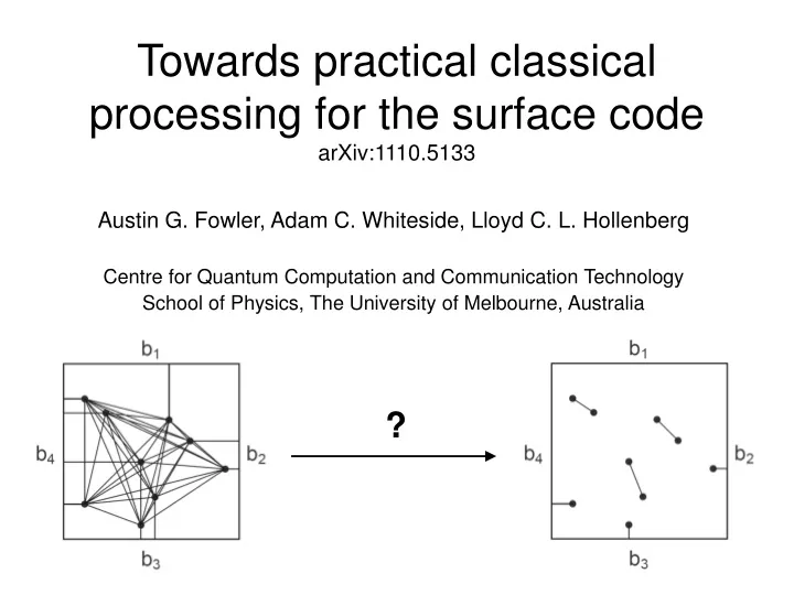
Towards practical classical processing for the surface codearXiv:1110.5133 Austin G. Fowler, Adam C. Whiteside, Lloyd C. L. Hollenberg Centre for Quantum Computation and Communication Technology School of Physics, The University of Melbourne, Australia ?
Overview • why study the surface code? • what is the surface code? • classical processing challenges • correcting errors fast enough • interpreting logical measurements • complexity optimal error processing • performance in detail • 3 second fault-tolerant distance 1000 • summary and further work
no known parallel arbitrary interaction quantum computer (QC) architecture many 2-D nearest neighbor (NN) architectures ion traps, superconducting circuits, quantum dots, NV centers, neutral atoms, optical lattices, electrons on helium, etc concatenated codes perform poorly on 2-D NN architectures Steane, Bacon-Shor pth~2x10⁻⁵ distance d = 9 Steane code currently requires 2304 qubits d = 27 requires 100k+ nq = d3.52 surface code performs optimally on a 2-D NN QC surface code has pth~10-2, so lower d required low overhead implementations of the entire Clifford group flexible, long-range logical gates distance 9 surface code currently requires 880 qubits distance 10 requires 1036 distance 27 requires 4356 nq = 6d2 lower overhead and 10x higher pth than any other known 2-D topological code Why study the surface code? The surface code is by far the most promising and practical code currently known.
a minimum of 13 qubits (13 cells) are required to create a single fault-tolerant surface code memory the nine circles store the logical qubit, the four dots are repeatedly used to detect errors on neighboring qubits an arbitrary single error can be corrected, multiple errors can be corrected provided they are separated in space or time in a full-scale surface code quantum computer, a minimum of 72 qubits are required per logical qubit the error correction circuitry is simple and transversely invariant Surface code: memory scalable logical qubit minimum-size logical qubit detect X error detect Z error order of interactions
when using error correction, only a small set of single logical qubit gates are possible for the surface code, these are, in order of difficulty, X, Z, H, S and T X and Z are applied within the classical control software H can be applied transversely after cutting the logical qubit out of the lattice S and T involve the preparation of ancilla states and gate teleportation the ancilla states must be distilled to achieve sufficiently low probability p of error an efficient, non-destructive S circuit exists, removing the need to reinject and redistill Y states Single logical qubit gates Hadamard after cutting (stop interacting with qubits outside the green square) ancilla state required for S ancilla state required for T state distillation p → 7p3 gate teleportation S, T, RZ() non-destructive S circuit
there are two types of surface code logical qubit, rough and smooth the simplest CNOT (CX) has smooth control and rough target CX can be defined by its effect on certain operators given a state XI = , CX = CXXI = CXXICXCX = XXCX XI→XX, IX→IX, ZI→ZI, IZ→ZZ defines CX moving (braiding) the holes (defects) that define logical qubits deforms their associated logical operators, performing computation movement is achieved by dynamically changing which data qubits are error corrected more complex braid patterns are required for rough-rough CX Surface code CNOT smooth-rough CNOT smooth qubit CNOT braid patterns rough qubit
stretching the braid pattern enables arbitrarily long-range CNOT the need to propagate error correction information near each braid prevents violations of relativity Clifford group computations can proceed without waiting for this information this enables CNOTs to be effectively bent backwards in time note that single control, multiple target CNOT is a simple braid pattern arbitrary Clifford group computations can be performed in constant time Long-range CNOT
correcting errors fast enough a single round of surface code QEC can involve as few as five sequential quantum gates depending on the underlying technology, this may take less than a microsecond need to be able to process a complex, infinite size graph problem in a very small constant time interpreting logical measurements surface code quantum computing is essentially a measurement based scheme logical gates, including the identity gate, introduce byproduct operators determining what these byproduct operators are is exceedingly difficult, especially after optimizing a braid pattern Classical processing challenges 4 1 2 5 3 7 6
consider the life cycle of a single error in the bulk of the lattice, a single gate error is always detected at two space-time points given a detailed error model for each gate, the probability that any given pair of space-time points will be connected by a single error can be calculated these probabilities can be represented by two lattices of cylinders recently completed open source tool to perform such error analysis and visualisation Correcting errors fast enough detect X error detect Z error
the primal (Z errors) and dual (X errors) lattices are independent deterministically constructed objects terminology: dots and lines weight of line –ln(pline) stochastically detected errors are represented by vertices associated with specific dots edges between vertices have weight equal to the minimum weight path through the lattice by choosing a minimum weight matching of vertices, corrections can be applied highly likely to preserve the logical state Correcting errors fast enough
minimum weight perfect matching was invented by Jack Edmonds in 1965 very well studied algorithm, however best publicly available implementations have complexity O(n3) for complete graphs don’t support continuous processing don’t support parallel processing actually quite slow as recently as this year [PRA 83, 020302(R) (2011)], distance ~ 10 was the largest surface code that had been studied fault-tolerantly renormalization techniques have been used to study large non-fault-tolerant surface codes [PRL 104, 050504 (2010), arXiv:1111.0831] need something much better if surface code quantum computer is to be built Correcting errors fast enough
to describe our fast matching algorithm, replace complex 3-D lattice with simple uniform weight 2-D lattice (grey lines) vertices (error chain endpoints) are represented by black dots matched edges are thick black lines shaded regions are space-time locations the algorithm has explored Correcting errors fast enough
Complexity optimal error correction choose a vertex
Complexity optimal error correction explore local space-time region until other objects encountered
Complexity optimal error correction if unmatched vertices encountered, match with one
Complexity optimal error correction choose another vertex
Complexity optimal error correction 1 2 expand until other objects are encountered, build alternating tree
Complexity optimal error correction 1 it alternating tree outer space-time regions can’t be expanded, form blossom
Complexity optimal error correction 1 uniformly expand space-time region around blossom until other objects encountered
Complexity optimal error correction 1 two options in this case, unmatched vertex or boundary, choose vertex
Complexity optimal error correction choose another vertex
Complexity optimal error correction 1 2 form alternating tree
Complexity optimal error correction 1 2 expand outer nodes, contract inner nodes
Complexity optimal error correction 1 form blossom
Complexity optimal error correction 1 2 grow alternating tree
Complexity optimal error correction 1 2 expand outer nodes, contract inner nodes, forbidden region entered
Complexity optimal error correction 1 2 undo expand outer, contract inner
Complexity optimal error correction undo grow alternating tree
Complexity optimal error correction undo form blossom
Complexity optimal error correction undo expand outer, contract inner... done until have additional data
Complexity optimal error correction • noteworthy features: • many rules, but each rule is simple and cheap • on average, each vertex only needs local information • fewer vertices = faster, simpler and more local processing • algorithm remains efficient at and above threshold • average runtime is O(n) per round of error correction • the runtime is independent of the amount of history, which can be discarded after a delay, finite memory required • algorithm can be parallelized to O(1) using constant computing resources per unit area (unit width in the example) • current implementation is single processor only
Performance in detail • we simulate surface codes of the form shown on the right • depolarizing noise of strength p is applied after every unitary gate, including the identity • measurement reports the wrong eigenstate with probability p but leaves the state in the reported eigenstate • for each d and p, our simulations continuously apply error correction until 10,000 logical errors have been observed • the probability of logical error per round of error correction is then calculated and plotted
Performance in detail 0.5 0.1 0.5% 0.2%
matching, while still efficient, is much slower around and above the threshold error rate very large blossoms appear at d = 55, p = 10-2, approximately 6 GB of memory required at an error rate p = 10-3, it is straightforward to simulate d = 1000 over 4 million qubits 3 seconds per round of error correction approximately 100 µs per vertex pair, at least 90% of that is memory access time parallelized, this would be sufficiently fast for many quantum computer architectures but not all... achieving sufficiently fast, high error rate, fault-tolerant, parallel surface code quantum error correction is extremely challenging without further work, classical processing speed will limit the maximum tolerable error rate Performance in detail
Summary and further work • complexity optimal algorithm • O(n2) serial • O(1) parallel • accurately handle general error models • sufficiently fast at p = 10-3 for many architectures • next 12 months: • parallelize the algorithm • benchmark on commercially available parallel computing hardware • reduce memory usage, improve core speed, raise practical p • take error correlations into account • develop algorithms capable of simulating braided logical gates • get building!