Download
1 / 38
410 likes | 565 Vues
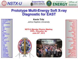
Design and tomography test of edge multi-energy s oft X-ray diagnostics on KSTAR. PPPL, Feb. 18, 2014. Juhyeok Jang *, Seung Hun Lee, H. Y. Lee, Joohwan Hong, Juhyung Kim, Siwon Jang, Taemin Jeon , Jae Sun Park and Wonho Choe **

E N D
Design and tomography test ofedge multi-energy soft X-ray diagnostics on KSTAR PPPL, Feb. 18, 2014 Juhyeok Jang*, Seung Hun Lee, H. Y. Lee, Joohwan Hong, JuhyungKim, SiwonJang, TaeminJeon, Jae Sun Park and WonhoChoe** Korea Advanced Institute of Science and Technology (KAIST), Daejeon, Korea Fusion Plasma Transport Research Center (FPTRC), Daejeon, Korea *jjh4368@kaist.ac.kr **wchoe@kaist.ac.kr
Outline • Motivation • Expected research topics • Engineering design • Installation position • Array design • Detector specification • Expected signal level & Tomography test • Calculation method • Test for trial ne, Te profiles • Test for KSTAR L, H-mode ne, Teprofiles • Time resolution test • Summary & Discussions
Motivation • Multi-energy soft X-ray (ME-SXR) • Tangential measurement • Multiple filter mode : bolometer, Be filters, etc • High spatial / time resolution : spatial ~ 1 cm, time > 10 kHz • Possible studies • Edge plasma physics : ELM, MHD instabilities • Edge electron temperature calculation by Neural Network NSTX* * Kevin Tritz, KAIST seminar (2013)
Edge plasma physics • High time resolution measurement of MHD activities • ELM cycle dynamics Comparison with ECEI results • Impurity transport SANCO calculation constrained by edge SXR signal Resistive Wall Mode (NSTX) * ELM filament (KSTAR ECEI) ** * L Delgado-Aparicio, Plasma Phys. Control. Fusion, 53 (2011) ** G. S. Yun, PRL 107, 045004 (2011)
Electron temperature measurement • Neural Network: Three layer technique • Fast, real-time data analysis • Te profile measurement without atomic modelling Three-layer Neural Network * Te measurement (NSTX) ** * Kevin Tritz, KAIST seminar (2013) ** D. J. Clayton, Plasma Phys. Control. Fusion, 55 (2013)
Engineering Design • Installation position • Viewing range • Array design • Detector specification
Installation position (1) poloidal tangential F-port • Poloidal edge array Tangential edge array • KSTAR F-port : possible location of tangential array design • Fixed boundary, higher signal level
Installation position (2) KSTAR top view F-port NBI armor F-port F-port Possible position • Position : KSTAR F-port
Viewing range Line of sight 30 - 50 cm from core (r/a = 0.6-1.0) F-port D-port • Range : r/a = 0.6~1.0 • Resolution ~ 1.3 cm
Array Design (1) NBI armor AXUV photodiode Welding plate KSTAR wall Preamp Sight guide KSTAR wall case NBI armor Sight line pinhole • 3 AXUV photodiodes • 1 bolometer mode, 2 Be filters • Preamp (106V/A) close to the detectors
Array Design (2) 1 1 2 2 • Array size : 400 mm 220 mm 120 mm • Pinhole–detector distance : 320 mm
Pinhole & Crosstalk 30 - 50 cm from core (r/a = 0.6-1.0) pinhole 19 mm 13 mm 3 mm • Pinhole : 5 mm 1 mm • Resolution ~ 13 mm • Cross talk ~ 3mm
Detector specification AXUV-16ELG photodiode Ribbon cable AXUV-16ELG array 15 mm 55 mm 53 mm t = 2 s r = 2 cm • Requirement • Fast response ~ MHz • High sensitivity to XUV and soft X-ray • Specification • Active area: 5 2 mm2 • Shunt resistance: 100 m • Capacitance: 2 nF • Rise time (10-90%): 0.5 s • Gain: 106 V/A • Detection efficiency: 0.27 A/W 73 mm AMP-16 remote panel AMP-16 main circuit
Expected signal level • & Tomography test • Filter selection • Calculation method • Expected signal & tomography test • trial ne, Te profiles • KSTAR L, H-mode ne, Te profiles • Filament structure calculation
Filter selection • Edge SXR : 3 mode • 1 bolometer mode (no filter) • 2 Be filter modes (Be 5 μm, 10 μm) • Cutoff energy of Be filters • Be 5 μm : 0.5 keV • Be 10 μm : 0.6 keV * Photo-current : transparency of filter : transparency of Si detector Be filter transparency bolometer Be 5 μm Be 10 μm
Calculation condition • KSTAR magnetic flux #7566, 2.0 s • Toroidal symmetry • Edge SXR chord • r/a = 0.6~1.0 • resolution ~ 1.3 cm • Continuum radiation • Brems. + Recomb. • Photon 0.1-100 keV • Mode • Bolometer, Be 5 μm, Be 10 μm Top view Poloidal view 3 cm
Solid angle calculation dPi: measured power emitted from the plasma volume dVp 5 × 2 mm2 322 mm di h Line of sight, Li 5 × 1 mm2 Detector, Adet,i Aperture, Aap,i Thickness, dli Plasma volume, dVp ci : calibration factor
Tomography Weight matrix flux j channel i • Intersection lengthbetween • sight line and magnetic flux surfaces • J = Laplacian+ mean squared error • /M • Solution minimizing J • : regularization parameter • GCV method Phillip-Tikhonov method
Tomography test sequence Input • ne, Te profile • Continuum radiation : • Edge SXR chord, flux surfaces • Weight matrix : W Signal level • Line integrated signal • Noise test • ( : random detection noise) Evaluation Output • Shape • Smoothness • error(%) • Phillips Tikhonov method • 1-D radial emissivity profile
Poloidalvs Tangential Poloidal Tangential Radiation • Condition • Same solid angle • Current level • tangential ~ 3poloidal • long integration length
Trial profiles ne, Te~ Core : ne = 41019m-3, Te = 2 keV profile 1 : a=2, b=0.4profile 2 : a=2, b=1 Electron density (1019m-3) Electron temperature (keV) • Signal level and tomography test with parabolic ne, Te profile
Continuum radiation Profile1 radiation (kW/m3) Profile2 radiation (kW/m3) Viewing range Viewing range
Expected photo-current Profile1 photo-current (μA) Profile2 photo-current (μA)
Tomography test (1) Be 5 μm Be 10 μm • Phatnom • Reconstruction • Phatnom • Reconstruction • Random noise test • : Chord signal + Random noise • Stability of reconstruction solution
Tomography test (2) Be 5 μm Be 10 μm • Phatnom • Reconstruction • Phatnom • Reconstruction • Reconstruction results agree with parabolic profiles.
KSTAR L, H-mode Electron density (1019m-3) Electron temperature (keV) • Signal level and tomography test with KSTAR L, H mode ne, Te profile
Continuum radiation L-mode radiation (kW/m3) H-mode radiation (kW/m3) Viewing range Viewing range
Expected photo-current L-mode photo-current (μA) H-mode photo-current (μA)
L-mode tomography test Be 5 μm Be 10 μm • Phatnom • Reconstruction • Phatnom • Reconstruction • Reconstruction results match with L-mode phantoms. • Reconstruction error increases with random detection noise.
H-mode tomography test Be 5 μm Be 10 μm • Phatnom • Reconstruction • Phatnom • Reconstruction • Pedestal structure is well reconstructed.
Filament structure calculation
ELM filament calculation D-shape Filament Phantom • Goal : possibility of investigation of • high frequency edge dynamics • ELM cycle dynamics • Edge MHD activity • Phantom • = ELM filament structure (m/n=8/1) • + toroidal rotation Toroidal rotation
Expected signal Line-integrated signal MHD activity in NSTX * • Line-integrated signal • : ~40 μs fluctuation observed • rotation velocity ~ 250 km/s • time resolution ~ 500 kHz (2 μs) • Signal change due to filament ~ 5 % • Possible studies • Possibility of high time resolution • (~500 kHz) measurement • Neural Network • fast Te fluctuation measurement * Kevin Tritz, KAIST seminar (2013)
Summary • Edge tangential soft X-ray design • KSTAR F-port • r/a = 0.6~1, spatial resolution ~ 1.3 cm • Three modes will be available (bolometer, Be 5 μm, Be 10 μm) • Expected photo-current level (bolometer, Be 5, 10 μm) • L-mode profile ~ 10 nA, 3.5 nA, 2.6 nA • H-mode profile ~ 70 nA, 36 nA, 30 nA • Tomography tests • Reconstruction results match with phantoms. • Error increases with random detection noise. • Filament structure calculation • ~ 40 μsfluctuation observation possible
Discussion • Signal level • Proper photo-current level for detection of edge soft X-ray • NSTX ME-SXR signal level : S/N ratio of AXUV 20ELG… • Optimized design for increasing signal level • Spatial resolution • Proper spatial resolution for investigation of edge plasma physics • Te calculation by Neural Network • Be filter selection for Neural Network method : energy range? • Mode number : 3 modes are enough? • Emissivity profile without tomography