Download
1 / 45
460 likes | 748 Vues
Analyzing Nonlinear Time Series with Hilbert-Huang Transform. Sai -Ping Li Lunch Seminar December 7, 2011. Introduction Hilbert-Huang Transform Empirical Mode Decomposition Some Examples and Applications Summary and Future Works. Some Examples of Wave Forms.

E N D
Analyzing Nonlinear Time Series with Hilbert-Huang Transform Sai-Ping Li Lunch Seminar December 7, 2011
Introduction • Hilbert-Huang Transform • Empirical Mode Decomposition • Some Examples and Applications • Summary and Future Works
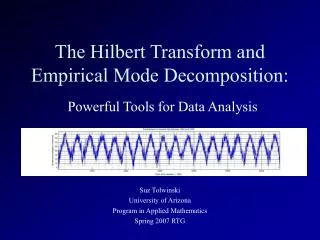
Time series: random data plus trend, with best-fit line and different smoothings
Examples of Non-Stationary Time Series Earthquake data of El Centro in 1985. Tidal data of Kahului Harbor, Maui, October 4-9, 1994. Difference of daily Non-stationary annual cycle and 30-year mean annual cycle of surface temperature at Victoria Station, Canada. Blood pressure of a rat.
Consider the non-dissipative Duffing equation: γ is the amplitude of a periodic forcing function with a frequency ω. If 𝜖 = 0, the system is linear and the solution can be found easily. If 𝜖 ≠ 0, the system becomes nonlinear. If 𝜖 is not small, perturbation method cannot be used. The system is highly nonlinear and new phenomena such as bifurcation and chaos can occur.
Rewrite the above equation as: The quantity in the parenthesis above can be regarded as a varying spring constant, or varying pendulum length. The frequency of the system can change from location to location, and also from time to time, even within one oscillation cycle.
Numerical Solution for the Duffing Equation Left: The numerical solution of x and dx/dt as a function of time. Right: The phase diagram with continuous winding indicates no fixed period of oscillations.
An Empirical data analysis method: Hilbert-Huang Transform Empirical Mode Decomposition (EMD) + Hilbert Spectral Analysis (HSA)
Empirical Mode Decomposition: Based on the assumption that any dataset consists of different simple intrinsic modes of oscillations. Each of these intrinsic oscillatory modes is represented by an intrinsic mode function (IMF) with the following definition: in the whole dataset, the number of extremaand the number of zero-crossings must either equal or differ at most by one, and (2) at any point, the mean value of the envelope defined by the local maxima and the envelope defined by the local minima is zero.
Example: A test Dataset Identify all local extrema, then connect all the local maxima by a cubic spline line in the upper envelope. Repeat the procedure for the local minima to produce the lower envelope. The upper and lower envelopes should cover all the data between them. Their mean is designated as .
The difference between the data and the mean is the first component , i.e., The data (blue) upper and lower envelopes (green) defined by the local maxima and minima, respectively, and the mean value of the upper and lower envelopes given in red. The data (red) and (blue).
Repeat the Sifting Process: Left: Repeated sifting steps with and . Right: Repeated sifting steps with and .
The Sifting Process for the first IMF: In the next step, Repeat Sifting, ● ● ● And is designated as,
Separate from the original data, and call the residue , The original data (blue) and the residue .
The procedure is repeated to get all the subsequent ’s , ● ● ● The original dataset is decomposed into a sum of IMF’s and a residue, Adecomposition of the data into n-empirical modes is achieved, and a residue obtained which can either be the mean trend or a constant.
A test dataset shown in the above. On the right is the original dataset decomposed into 8 IMF’s and a trend ().
Composition: LME monthly gold prices • Dividing the components into high, low and trend by reasonable boundary (12 months), and analyze the factors or economic meanings in different time scales. • Boundary: 12 months
Trend: inflation • We assume the gold price trend relates to inflation at first. • US monthly CPI and PPI are used to quantify the ordering of inflation. • Since the gold price trend hold high correlation with trend of CPI and PPI, the • economic meanings of trend can be described by “inflation”.
1979/11~1980/01: Iranian hostage crisis 1996 to 2006: Booming economic in USA 1987/10: New York Stock Market Crash 1980/09: Iran/Iraq War 1982/08: Mexico External Debt Crisis 2007/02: USA Subprime Mortgage Crisis 1973/10: 4th Middle East War 2008/09: Lehman Brothers bankruptcy Low frequency term: significant events • The six obvious variations correspond to six significant events. • The six significant events include wars, panic international situation, and financial crisis.
Example: Electroencephalography (EEG) and Heart Rate Variability (HRV)
Example: Electroencephalography (EEG) Active Wake Stage
Example: Electroencephalography (EEG) Stage I: Light Sleep Stage II Stage III Slow Wave Sleep Stage IV Quiet Sleep
Example: Electroencephalography (EEG) Left: A dataset of active wake stage. Right: Its corresponding IMF’s after EMD.
Example: Heart Rate Variability (HRV) Left: Original dataset Right: HRV after EMD
Relation of EEG and HRV of an Obstructive Sleep Apnea (OSA) patient using EMD analysis
Partial List of Application of HHT • Biomedical applications: Huang et al. [1999] • Chemistry and chemical engineering: Phillips et al. [2003] • Financial applications: Huang et al. [2003b] • Image processing: Hariharan et al. [2006] • Meteorological and atmospheric applications: Salisbury and Wimbush [2002] • Ocean engineering:Schlurmann [2002] • Seismic studies: Huang et al. [2001] • Solar Physics: Barnhart and Eichinger [2010] • Structural applications: Quek et al. [2003] • Health monitoring: Pines and Salvino [2002] • System identification: Chen and Xu [2002]
Problems related to Hilbert-Huang Transform Adaptive data analysis methodology in general (2) Nonlinear system identification methods (3) Prediction problem for non-stationary processes (end effects) (4) Spline problems (best spline implementation for the HHT, convergence and 2-D) (5) Optimization problems (the best IMF selection and uniqueness) (6) Approximation problems (Hilbert transform and quadrature) (7) Other miscellaneous questions concerning the HHT…….
Application: Price Fluctuations in Financial Time SeriesAll parameters are time dependent. is the drift, is the volatility and is a standard Wiener process with zero mean and unit rate of variance.
Stoppage Criterion: The criterion to stop the sifting of IMF’s. Historically, there are two methods: The normalized squared difference between two successive sifting operations defined as If this squared difference is less than a preset value, the sifting process will stop. (2) The sifting process will stop only after S consecutive times, when the numbers of zero-crossings and extrema stay the same and are equal or differ at most by one. The number S is preset.
Orthogonality: The orthogonality of the EMD components should also be checked a posteriori numerically as follows: let us first write equation as Form the square of the signal as And define IO as If the IMF’s are orthogonal, IO should be zero.