Download
1 / 35
360 likes | 641 Vues
Minkowski Sums and Distance Computation. Eric Larsen COMP 290-72 11-24-98. Minkowski Sums and Differences. Minkowski Sum (A, B) = { a + b | a A, b B } Minkowski Difference (A,B) = { a - b | a A, b B } = Minkowski Sum (A, -B)

E N D
Minkowski Sums and Distance Computation Eric Larsen COMP 290-72 11-24-98
Minkowski Sums and Differences • Minkowski Sum (A, B) = { a + b | a A, b B } • Minkowski Difference (A,B) = { a - b | a A, b B } = Minkowski Sum (A, -B) • A and B collide iff Minkowski Difference(A,B) contains the point 0.
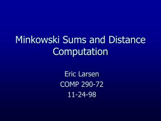
Some Minkowski Differences A B B A
Minkowski Difference and Translation • Minkowski Diff.(Translated(A,t1), Translated(B, t2)) = Translated (Minkowski Diff.(A,B), t1 - t2) • Translated(A, t1) and Translated(B, t2) intersect iff Minkowski Diff(A,B) contains point t2 - t1. • An example seen last time: • Robot translated from origin by x intersects Environment iff x Minkowski Diff(Environment, Robot)
Other Properties • Distance: • distance(A,B) = mina A, b B || a - b ||2 • distance(A,B) = min c Minkowski-Difference(A,B) || c ||2 • if A and B disjoint, c is point on boundary of Minkowski difference • Intersection-Depth: • intersection-depth(A,B) = min{ || t ||2 | A Translated(B,t) = } • intersection-depth(A,B) = mintMinkowski-Difference(A,B) || t ||2 • if A and B intersecting, t is point on boundary of Minkowski difference
Practicality • Expensive to compute boundary of Minkowski difference: • For convex polyhedra, Minkowski difference may take O(n2) • For general polyhedra, no known algorithm of complexity less than O(n6) is known • Yet, no better approach is known for true intersection depth • Distance is more promising. Minkowski differences are not the only theory applied to this problem.
GJK Method for Convex Polyhedra • GJK-DistanceToOrigin ( P ) // dimension is m • 1. Initialize P0 with m+1 or fewer points. • 2. k = 0 • 3. while (TRUE) { • 4. if origin is within CH( Pk ), return 0 • 5. else { • 6. find x CH(Pk) closest to origin, and Sk Pk s.t. x CH(Sk) • 7. see if any point p-x in P more extremal in direction -x • 8. if no such point is found, return |x| • 9. else { • 10. Pk+1 = Sk {p-x} • 11. k = k + 1 • 12. } • 13. } • 14. }
GJK - Running Time • Each iteration of the while loop requires O(n) time. • O(n) iterations possible, but authors claim between 3 and 6 iterations on average for any problem size, making this “expected” linear. • Trivial O(n) algorithms exist if we are given the boundary representation of a convex object, but GJK will work on point sets - computes CH lazily.
GJK - Two Convex Objects • A = CH(A’) A’ = { a1, a2, ... , an } • B = CH(B’) B’ = { b1, b2, ... , bm } • Minkowski-Diff(A,B) = CH(P), P = {a - b | a A’, b B’} • Thus, GJK-DistanceToOrigin(P) will find distance(A, B), but P has m*n points. • Can compute points of P on demand: • p-x = a-x - bx where a-x is the point of A’ extremal in direction -x, and bx is the point of B’ extremal in direction x. • The loop body would now take O(n + m) time, producing the same “expected” linear performance overall.
Lin-Canny Method for Convex Polyhedra • Observations: • for “smoothly” transforming convex objects, closest points may change little in successive frames - notion of coherence. • it is possible to confirm that two features (edges, vertices, faces) are the closest points of two convex objects in constant time, given some preprocessing of the polyhedra. • Method: • track closest points • after each transformation, make expected constant time adjustment of closest points
Voronoi Regions • Localized verification of closest features made possible by precomputing an external Voronoi diagram for the polyhedron • External Voronoi diagram - divide space outside polyhedron into regions, such that points inside each region are closest to a corresponding “feature” - a face, edge, or vertex - of the polyhedron.
Lin-Canny Algorithm • Given one feature from each polyhedron, find the closest points of the two features. If each point is in the Voronoi region of the other feature, closest features have been found. (more on this later)
Lin-Canny Algorithm • Otherwise, one of the points (call its feature F) is in the Voronoi region of another feature F’, and therefore closer to it. Can select F and F’ as next candidate feature pair.
Lin-Canny Running Time • Distance strictly decreases with each change of feature pair, and no pair of features can be selected twice. • Worst case O(n2) pairs checked. • Convergence to closest pair typically better: • O(1) achievable in simulations with coherence. • Closer to O(n) even without coherence.
Proof of Local Verification • Definition: for two points a and b, slab(a,b) is the slab bounded by parallel planes, one through a and another through b, both with normal a - b a slab(a,b) b
Proof of Local Verification • Claim: for two convex point sets A and B, points a A and b B are closest slab(a,b) has empty interior. a slab(a,b) c b
Proof of Local Verification • Proof: • : • suppose a and b are closest, but that slab(a, b) has nonempty interior. • Pick an arbitrary point inside slab(a,b), c which belongs to one of the point sets. Suppose it belongs to A. By convexity of A, line segment ca is inside A. Some point on ca is closer to b than a. Contradiction. • : given all points of A and B outside or on surface of slab, length || a - b ||2 is a lower bound.
Proof of Local Verification • Local verification steps: • step 1: find closest points a, b on two features fa, fb. • step 2: verify each point is inside other feature’s Voronoi region - i.e. each point not in the Voronoi region of another feature. • Need to show this is sufficient to verify closest points on polyhedra A and B are a and b.
Proof of Local Verification • By above claim, could do this by showing all points of polyhedra A and B are outside or on slab(a,b). • first fa and fb are convex and therefore on or outside slab(a,b). • What if some point, from A for example, inside the slab(a,b)? Provided A and B do not overlap, there would be some boundary point of A closer to b than a, implying b closer to some other feature f than fa, and inside Voronoi(f). Contradiction.
Distance for General Models • Many local minima make distance more complicated for non-convex models: • Discontinuous change of closest features with transformations • When a local minimum is found, no longer able to disregard rest of the model
Methods for General Models • Decompose into convex pieces, and take minimum over all pairs of pieces: • Optimal (minimal) model decomposition is NP-hard. • Approximation algorithms exist for closed solids, but what about a list of triangles? • Decompose into triangles: • n*m pairs of triangles - brute force expensive • Bounding volume hierarchies used to accelerate minimum finding
Hierarchical Collision Detection • Model Hierarchy: • each node has a simple volume that bounds a set of triangles. • children contain volumes that each bound a different portion of the parent’s triangles. • The leaves of the hierarchy usually contain individual triangles. • A binary bounding volume hierarchy:
Hierarchical Collision Detection • 1. Recursive-Collide(BV a, BV b) { • 2. if (! bv-overlap(a,b)) return; • 3. if (leaf(a) && leaf(b)) { • 4. tri-overlap(tri(a), tri(b)) • 5. } • 6. else if (!leaf(a)) { • 7. Recursive-Collide(lchild(a), b) • 8. Recursive-Collide(rchild(a), b) • 9. } • 10. else { • 11. Recursive-Collide(a, lchild(b)) • 12. Recursive-Collide(a, rchild(b)) • 13. } • 14. }
Hierarchical Distance Computation • Test at least one pair of triangles to get a “candidate” minimum distance. • Recursion terminates when distance between bounding volumes > candidate minimum distance. • Differences from collision detection: • mandatory visitation of leaf nodes • wider search tree • BV distance generally more expensive than overlap
Quinlan’s Approach • Hierarchy building: • Uses spheres as bounding volume • First tiles surface of triangles with many small spheres, so that many leaf nodes may have a pointer to the same triangle. • Builds a hierarchy top down that bounds these spheres, instead of triangles.
Quinlan’s Approach • Distance Computation: • Same method as previously outlined, except that many leaf node pairs may correspond to same triangle. • Triangle pair distances are hashed to avoid redundant computations. • Quinlan’s code is currently the fastest in practice for general models. • Tiling may be most critical factor.
Quinlan’s Approach • Distance Computation: • Same method as previously outlined, except that many leaf node pairs may correspond to same triangle. • Triangle pair distances are hashed to avoid redundant computations. • Quinlan’s code is currently the fastest in practice for general models. • Tiling may be most critical factor.
Quinlan’s Approach • Distance Computation: • Same method as previously outlined, except that many leaf node pairs may correspond to same triangle. • Triangle pair distances are hashed to avoid redundant computations. • Quinlan’s code is currently the fastest in practice for general models. • Tiling may be most critical factor.
Quinlan’s Approach • Distance Computation: • Same method as previously outlined, except that many leaf node pairs may correspond to same triangle. • Triangle pair distances are hashed to avoid redundant computations. • Quinlan’s code is currently the fastest in practice for general models. • Tiling may be most critical factor.
Conclusions • Minkowski Difference is useful theory but costly to compute explicitly. • Not only applicable theory to distance computation, as evidenced by Lin-Canny and hierarchical methods • Coherence not yet exploited for non-convex models - hierarchical methods currently most useful.
References • Computing the Intersection-Depth of Polyhedra - Dobkin, Hershberger, Kirkpatrick, Suri • A Fast Procedure for Computing the Distance Between Complex Objects in Three-Dimensional Space - Gilbert, Johnson, Keerthi 1988 • Efficient Collision Detection for Animation and Robotics - Ming Lin 1994 • Efficient Distance Computation between Non-Convex Objects - Sean Quinlan 1994