Download

1 / 14
140 likes | 242 Vues
Dive into the intricacies of linear-time sorting algorithms such as Counting Sort, Radix Sort, and Bucket Sort. Learn their key assumptions, implementation details, and stability characteristics.

E N D
Sorting in Linear Time Comp 550, Spring 2015
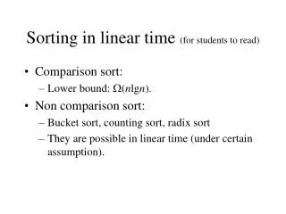
Linear-time Sorting • Depends on a key assumption: numbers to be sorted are integers in {0, 1, 2, …, k}. • Input: A[1..n] , where A[j] {0, 1, 2, …, k} for j = 1, 2, …, n. Array A and values n and k are given as parameters. • Output:B[1..n] sorted. B is assumed to be already allocated and is given as a parameter. • Auxiliary Storage:S[0..k] • Runs in linear time if k = O(n). • Example: On board. Comp 550, Spring 2015
Counting-Sort (A, B, k) CountingSort(A, B, k) 1. fori 0 to k 2. doS[i] 0 3. forj 1 to length[A] 4. doS[A[j]] S[A[j]] + 1 5. fori 1 to k 6. doS[i] S[i] + S[i –1] 7. forjlength[A] downto 1 8. doB[S[A[ j ]]] A[j] 9. S[A[j]] S[A[j]]–1 O(k) No comparisons made: it uses actual values of the elements to index into an array. O(n) O(k) O(n) The overall time is O(n+k). When we have k=O(n), the worst case is O(n). Comp 550, Spring 2015
Stableness • Stable sorting algorithms maintain the relative order of records with equal keys (i.e. values). That is, a sorting algorithm is stable if whenever there are two records R and S with the same key and with R appearing before S in the original list, R will appear before S in the sorted list. Comp 550, Spring 2015
Radix Sort • It is the algorithm for using the machine that extends the technique to multi-column sorting. • Key idea: sort on the “least significant digit” first and on the remaining digits in sequential order. The sorting method used to sort each digit must be “stable”. Comp 550, Spring 2015
An Example After sorting on LSD After sorting on MSD After sorting on middle digit Input 392 631 928 356 356 392 631 392 446 532 532 446 928 495 446 495 631 356 356 532 532 446 392 631 495 928 495 928 Comp 550, Spring 2015
Radix-Sort(A, d) RadixSort(A, d) 1. for i 1 to d 2. do use a stable sort to sort array A on digit i Correctness of Radix Sort By induction on the number of digits sorted. Assume that radix sort works for d – 1 digits. Show that it works for d digits. Radix sort of d digits radix sort of the low-order d– 1 digits followed by a sort on digit d . Comp 550, Spring 2015
Correctness of Radix Sort By induction hypothesis, the sort of the low-order d – 1 digits works, so just before the sort on digit d , the elements are in order according to their low-order d – 1 digits. The sort on digit d will order the elements by their dth digit. Consider two elements, a and b, with dth digits adand bd: • If ad< bd , the sort will place a before b, since a < b regardless of the low-order digits. • If ad> bd , the sort will place a after b, since a > b regardless of the low-order digits. • If ad= bd , the sort will leave a and b in the same order, since the sort is stable. But that order is already correct, since the correct order of is determined by the low-order digits when their dth digits are equal. Comp 550, Spring 2015
Algorithm Analysis • Each pass over n d-digit numbers then takes time (n+k). (Assuming counting sort is used for each pass.) • There are d passes, so the total time for radix sort is(d (n+k)). • When d is a constant and k = O(n), radix sort runs in linear time. Comp 550, Spring 2015
Bucket Sort • Assumes input is generated by a random process that distributes the elements uniformly over [0, 1). • Idea: • Divide [0, 1) into n equal-sized buckets. • Distribute the n input values into the buckets. • Sort each bucket. • Then go through the buckets in order, listing elements in each one. Comp 550, Spring 2015
An Example Comp 550, Spring 2015
Bucket-Sort (A) Input:A[1..n], where 0 A[i] < 1 for all i. Auxiliary array:B[0..n – 1] of linked lists, each list initially empty. BucketSort(A) 1. n length[A] 2. fori 1 to n 3. do insert A[i] into list B[ nA[i] ] 4. fori0ton – 1 5. do sort list B[i] with insertion sort • concatenate the lists B[i]s together in order • return the concatenated lists Comp 550, Spring 2015
Correctness of BucketSort • Consider A[i], A[j]. Assume w.o.l.o.g, A[i] A[j]. • Then, n A[i] n A[j]. • So, A[i] is placed into the same bucket as A[j] or into a bucket with a lower index. • If same bucket, insertion sort fixes up. • If earlier bucket, concatenation of lists fixes up. Comp 550, Spring 2015
Analysis • Relies on no bucket getting too many values. • All lines except insertion sorting in line 5 take O(n) altogether. • Intuitively, if each bucket gets a constant number of elements, it takes O(1) time to sort each bucket O(n) sort time for all buckets. • We “expect” each bucket to have few elements, since the average is 1 element per bucket. • But we need to do a careful analysis. Comp 550, Spring 2015