Download
1 / 31
310 likes | 387 Vues
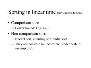
Sorting in Linear Time. Lower bound for comparison-based sorting Counting sort Radix sort Bucket sort. Sorting So Far. Insertion sort: Easy to code Fast on small inputs (less than ~50 elements) Fast on nearly-sorted inputs O(n 2 ) worst case O(n 2 ) average (equally-likely inputs) case

E N D
Sorting inLinear Time Lower bound for comparison-based sorting Counting sort Radix sort Bucket sort
Sorting So Far Insertion sort: • Easy to code • Fast on small inputs (less than ~50 elements) • Fast on nearly-sorted inputs • O(n2) worst case • O(n2) average (equally-likely inputs) case • O(n2) reverse-sorted case
Sorting So Far • Merge sort: • Divide-and-conquer: • Split array in half • Recursively sort subarrays • Linear-time merge step • O(n lg n) worst case • Doesn’t sort in place
Sorting So Far • Heap sort: • Uses the very useful heap data structure • Complete binary tree • Heap property: parent key > children’s keys • O(n lg n) worst case • Sorts in place • Fair amount of shuffling memory around
Sorting So Far • Quick sort: • Divide-and-conquer: • Partition array into two subarrays, recursively sort • All of first subarray < all of second subarray • No merge step needed! • O(n lg n) average case • Fast in practice • O(n2) worst case • Naïve implementation: worst case on sorted input • Address this with randomized quicksort
How Fast Can We Sort? • First, an observation: all of the sorting algorithms so far are comparison sorts • The only operation used to gain ordering information about a sequence is the pairwise comparison of two elements • Comparisons sorts must do at least n comparisons (why?) • What do you think is the best comparison sort running time?
Decision Trees • Abstraction of any comparison sort. • Represents comparisons made by • a specific sorting algorithm • on inputs of a given size. • Abstracts away everything else: control and data movement. • We’re counting only comparisons. • Each node is a pair of elements being compared • Each edge is the result of the comparison (< or >=) • Leaf nodes are the sorted array
Insertion Sort 4 Elements as a Decision Tree Compare A[1] and A[2] Compare A[2] and A[3]
The Number of Leaves in a Decision Tree for Sorting Lemma:A Decision Tree for Sorting must have at least n! leaves.
Lower Bound For Comparison Sorting • Thm: Any decision tree that sorts n elements has • height (n lg n) • If we know this, then we know that comparison sorts are always (n lg n) • Consider a decision tree on n elements • We must have at least n! leaves • The max # of leaves of a tree of height h is 2h
Lower Bound For Comparison Sorting • So we have… n! 2h • Taking logarithms: lg (n!) h • Stirling’s approximation tells us: • Thus:
Lower Bound For Comparison Sorting • So we have • Thus the minimum height of a decision tree is (n lg n)
Lower Bound For Comparison Sorts • Thus the time to comparison sort n elements is (n lg n) • Corollary: Heapsort and Mergesort are asymptotically optimal comparison sorts • But the name of this lecture is “Sorting in linear time”! • How can we do better than (n lg n)?
Counting Sort – Sort small numbers • Why it’s not a comparison sort: • Assumption: input - integers in the range 0..k • No comparisons made! • Basic idea: • determine for each input element x its rank: the number of elements less than x. • once we know the rank r of x, we can place it in position r+1
Counting SortThe Algorithm • Counting-Sort(A) • Initialize two arrays B and C of size n and set all entries to 0 • Count the number of occurrences of every A[i] • fori = 1..n • do C[A[i]] ← C[A[i]] + 1 • Count the number of occurrences of elements <= A[i] • fori = 2..n • do C[i] ← C[i] + C[i – 1] • Move every element to its final position • fori = n..1 • do B[C[A[i]] ←A[i] • C[A[i]] ← C[A[i]] – 1
1 2 3 4 5 6 7 8 0 3 2 5 3 0 2 3 A = 0 1 2 3 4 5 C = 2 0 2 3 0 1 1 2 3 4 5 6 7 8 3 B = 0 1 2 3 4 5 7 C = 2 2 4 7 8 6 Counting Sort Example 0 1 2 3 4 5 C = 2 2 4 7 7 8
1 Counting Sort Example 1 2 3 4 5 6 7 8 0 3 2 5 3 0 2 3 A = 0 1 2 3 4 5 C = 2 2 4 6 7 8 1 2 3 4 5 6 7 8 3 0 B = 0 1 2 3 4 5 C = 2 2 4 6 7 8
5 Counting Sort Example 1 2 3 4 5 6 7 8 0 3 2 5 3 0 2 3 A = 0 1 2 3 4 5 C = 2 2 4 6 7 8 1 2 3 4 5 6 7 8 3 3 0 B = 0 1 2 3 4 5 C = 1 2 4 6 7 8
Takes time O(k) Takes time O(n) Counting Sort 1 CountingSort(A, B, k) 2 for i=1 to k 3 C[i]= 0; 4 for j=1 to n 5 C[A[j]] += 1; 6 for i=2 to k 7 C[i] = C[i] + C[i-1]; 8 for j=n downto 1 9 B[C[A[j]]] = A[j]; 10 C[A[j]] -= 1; What will be the running time?
Counting Sort • Total time: O(n + k) • Usually, k = O(n) • Thus counting sort runs in O(n) time • But sorting is (n lg n)! • No contradiction--this is not a comparison sort (in fact, there are no comparisons at all!) • Notice that this algorithm is stable • If numbers have the same value, they keep their original order
Input 21 71 41 42 22 51 23 61 Output 21 22 23 41 42 51 61 71 Stable Sorting Algorithms • A sorting algorithms is stable if for any two indices i and j with i < j and ai = aj, element ai precedes element aj in the output sequence. Observation:Counting Sort is stable.
Counting Sort • Linear Sort! Cool! Why don’t we always use counting sort? • Because it depends on range k of elements • Could we use counting sort to sort 32 bit integers? Why or why not? • Answer: no, k too large (232 = 4,294,967,296)
Radix Sort • Why it’s not a comparison sort: • Assumption: input has d digits each ranging from 0 to k • Example: Sort a bunch of 4-digit numbers, where each digit is 0-9 • Basic idea: • Sort elements by digit starting with least significant • Use a stable sort (like counting sort) for each stage
Radix SortThe Algorithm • Radix Sort takes parameters: the array and the number of digits in each array element • Radix-Sort(A, d) • 1fori = 1..d • 2do sort the numbers in arrays A by their i-th digit from the right, using a stable sorting algorithm
Radix SortCorrectness and Running Time • What is the running time of radix sort? • Each pass over the d digits takes time O(n+k), so total time O(dn+dk) • When d is constant and k=O(n), takes O(n) time • Stable, Fast • Doesn’t sort in place (because counting sort is used)
Bucket Sort • Assumption: input - n real numbers from [0, 1) • Basic idea: • Create n linked lists (buckets) to divide interval [0,1) into subintervals of size 1/n • Add each input element to appropriate bucket and sort buckets with insertion sort • Uniform input distribution O(1) bucket size • Therefore the expected total time is O(n)
Bucket Sort Bucket-Sort(A) • n length(A) • fori 0 to n • do insert A[i] into list B[floor(n*A[i])] • fori 0 to n –1 • do Insertion-Sort(B[i]) • Concatenate lists B[0], B[1], … B[n –1] in order Distribute elements over buckets Sort each bucket
.12 .17 .21 .23 .26 .39 .68 .72 .78 .94 Bucket Sort Example 0 1 .12 .17 2 .21 .23 .26 3 .39 4 5 6 .68 7 .72 .78 8 9 .94
Bucket Sort – Running Time • All lines except line 5 (Insertion-Sort) take O(n) in the worst case. • In the worst case, O(n) numbers will end up in the same bucket, so in the worst case, it will take O(n2) time. • Lemma:Given that the input sequence is drawn uniformly at random from [0,1), the expected size of a bucket is O(1). • So, in the average case, only a constant number of elements will fall in each bucket, so it will takeO(n) • Use a different indexing scheme (hashing) to distribute the numbers uniformly.
Summary • Every comparison-based sorting algorithm has to takeΩ(n lg n) time. • Merge Sort, Heap Sort, and Quick Sort are comparison-based and take O(n lg n) time. Hence, they are optimal. • Other sorting algorithms can be faster by exploiting assumptions made about the input • Counting Sort and Radix Sort take linear time for integers in a bounded range. • Bucket Sort takes linear average-case time for uniformly distributed real numbers.