Foreign Exchange Rate Determinants and International Parity Conditions

1. Foreign Exchange Rate Determinants and International Parity Conditions

2. Exchange Rate Determinants Questions: 1. What are the determinants of exchange rates? • Exchange rates are determined by the demand and supply of one currency relative to the demand and supply of another 2. Are changes in exchange rates predictable?

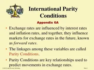
3. Exchange Rate Determinants • There are no general theory of exchange rate determination • Parity Condition, an economic theory, attempts to explain long-run exchange rate determinants • Other numerous variables attempt to explain short-run • The same set determinants will not, however, apply for all countries at all times

4. Potential Foreign Exchange Rate Determinants Parity condition 1. Relative inflation rate (PPP) 2. Relative interest rate (Fisher effect and real interest differential 3. Forward exchange rate 4. Exchange rate regimes 5. Monetary reserves Infrastructure 1. Strength of banking system 2. Strength of securities market 3. Outlook to growth and profitability Spot Exchange Rate Speculation 1. Currencies 2. Securities 3. Uncovered interest arbitrage 4. Real estate 5. Commodities Political Risk 1. Capital control 2. Black market 3. Exchange rate spreads 4. Risk premium on securities and FDI Cross-Boarder Investment 1. FDIs 2. Portfolio Investment

5. The BOP Approach • The BOP helps forecast a country’s market potential, esp. in the short run. (Note: A country experiencing a serious BOP deficit would not likely expand imports.) • The BOP is an important indicator of pressure on a country’s exchange rate – may spell foreign exchange gain or loss, for firm trading or investing in that country. • Changes in a country’s BOP may signal imposition (or removal) of controls over payment of dividends or interest, license fees, royalty fees, or other cash disbursements to foreign firms or investors.

6. The BOP Approach • Fixed Exchange Rate Countries • the government bears the responsibility to ensure a near zero BOP • the government is expected to intervene by buying or selling foreign exchange reserves, if the sum of the Current and Capital Accounts does not approximate to zero • if the Overall Balance is greater than zero, a surplus demand for the domestic currency exists in the world. The government must sell domestic currency for foreign currencies or gold. • if deficit, the government then must buy domestic currency for foreign currencies or gold.

7. The BOP Approach • Floating Exchange Rate Countries • the government has no responsibility to peg the foreign exchange rate • The fact that if the Overall Balance does not sum to zero will, in theory, automatically alter the exchange rate in the direction necessary to obtain a near zero BOP. • Example: A deficit in BOP means an excess supply of the domestic currency in the world market appears. As in the case with all goods in excess supply, the market lowers the price. Thus, the domestic currency will fall in value, and the BOP will move back towards zero. • The exchange rate markets do not always follow this theory, particularly in the short- to intermediate term.

8. The BOP Approach • Managed Float Exchange Rate Countries • the government still relies on market conditions for day-to-day exchange rate determination. • Necessary to take actions to maintain their desired exchange rate values by influencing the motivations of market activity, rather than through direct intervention. • The primary action taken is to change relative interest rates, thus influencing the economic fundamentals. This is an attempt to alter CI-CO, especially the short-term portfolio. • Raising domestic interest rates may attract additional capital from abroad.

9. The Asset Market Approach • Today, only about 2% of all Fx transactions are related to the financing of imports/exports. • This suggests that 98% of Fx transactions are attributable to assets being traded in the global market. (Note: Assets denote treasury securities, corporate bonds, bank accounts, stocks, and real properties.) • The asset-market approach suggests that the decision for foreigners (or willingness of foreigners) to hold claims in monetary form depends partly on relative real interest rates and also on a country’s outlook for economic growth and profitability.

10. The Asset Market Approach • The approach assumes instantaneous and continuous portfolio equilibrium and that E/R are modeled as being determined by the conditions for international asset market equilibrium. • Many economists reject the view that the short-term behavior of E/R is determined in flow markets. E/R are asset prices traded in an efficient financial market and therefore is determined by the willingness to hold each currency. • Like other asset prices, E/R is determined by expectations about the future, not current trade flows.

11. The Asset Market Approach • Example: During 1981– ‘85, the US dollar strengthened despite growing account deficits. This strength was due partly to relatively high real interest rates in the US. Another factor, however, was the heavy inflow of foreign capital into the US stock market and real estate, motivated by good long-run prospects for growth and profitability in the US.

12. Prices, Interest Rates, and Exchange Rates in Equilibrium • Using the Japanese yen as an example - 1. Exchange Rates: a. Current spot rate: ¥ 104/$ b. Forward rate (1 year): ¥ 100/$ c. Expected spot rate: ¥ 100/$ d. Forward premium on yen: 4% FY = S0– F x 100 = 104–100 x 100 = 4% F 100 e. Forecast change in spot rate: 4% %S = S0– S1 x 100 = 104–100 x 100 = 4% S1 100

13. Prices, Interest Rates, and Exchange Rates in Equilibrium 2. Forecast Rate of Inflation: a. Japan 1% b. USA 5% c. Difference -4% 3. Interest on 1-year GS a. Japan 4% b. USA 8% c. Difference -4%

14. International Parity Relations in Equilibrium Forward rate as an unbiased predictor (E) Forecast change in spot exchange rate +4% (yen strengthens) PPP (A) Forward premium on foreign currency +4% (yen strengthens) Forecast difference in rates of inflation -4% (less in Japan) International Fisher Effect (C) Interest Rate Parity (D) Difference in nominal interest rates -4% (less in Japan) Fisher Effect (B)

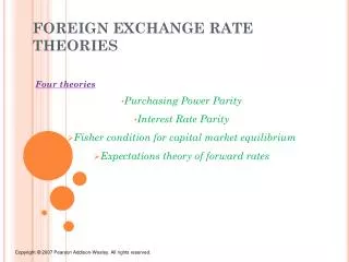
15. Economic Theories of Exchange Rate Determination • Price and exchange rates: • Law of One Price • Purchasing Power Parity (PPP) - Absolute Version - Relative Version • Real Exchange Rate (RER) • Exchange Rate Pass-Through • Money Supply and Price Inflation

16. Economic Theories of Exchange Rate Determination • Interest rate and exchange rates: • International Fisher Effect • Fisher Effect • Interest Rate Parity • Unbiased Forward Rates • Investor psychology and “Bandwagon” effects

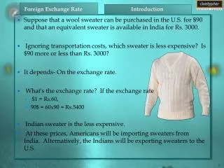
17. Law of One Price • In a competitive market that is free of transportation costs and trade barriers, identical products which are sold in different countries must sell for the same price when their price is expressed in terms of the same currency. • Example: US-France exchange rate is $1.2821/€. A jacket selling for €39 in Paris should retails for $50 (€39 x $1.2821/€) in New York. • Formula: P€ x S = P$

18. Law of One Price If the prices of the two products were stated in local currencies, the exchange rate could be deduced to: Formula (Derivation): Spot Rate (S0) = PH PF Where: Spot rate (S0) = Exchange rate PH = Price in home country PF = Price in foreign country In the Law of One Price, if a country’s currency depreciates, its counter-party must lower its price by a similar percentage. HCE/R50% = FCPrice 50%

19. Illustration: • If 1 ton of steel would be sold in the US and Japan, bearing the following prices, what should be the exchange rate according to the Law of One Price formula? Answer: ¥100/$ (2) If yen depreciated by 50% to ¥200/$, what should American and Japanese firms do? Answer: American firms should lower their price by 50%. Japanese firms should do nothing.

20. Rationale: Yen depreciated by 50% and is now ¥200/$ In Japan In the US Since the yen depreciated by 50%, American firms should lower their price by 50%, to be competitive.

21. Purchasing Power Parity • If the Law of One Price were true for all goods and services, the PPP exchange rate could be found from any individual set of prices. • By comparing the prices of identical products in different currencies, it should be possible to determine the ‘real’ or PPP exchange rate - if markets were efficient. • In relatively efficient markets (few impediments to trade and investment) then a ‘basket of goods’ should be roughly equivalent in each country.

22. Implied PPP • Formula: Implied PPP = PHC PFC where: PHC – price in home country PFC – price in foreign country • Deviation of the Implied PPP from the actual exchange rate (S0): Implied PPP – 1 = +/(–) S0 • If result is positive (+) , local currency is overvalued • If result is negative (+), local currency is undervalued

23. The Big Mac Index: PPP and Law of One Price Big Mac Prices Local Currency % Over(+) or Under(-) Valuation Against Dollar Price in Local Currency Actual Exchange Rate Implied PPP Price in Dollars Countries United States $2.49 2.49 - - - Argentina P 2.50 2.91 1.0040 0.8585 17 (O) Brazil R 3.60 1.54 1.4458 1.2415 16 (O) Canada C$ 3.33 2.90 1.3373 1.5783 - 15 (U) Euro € 2.67 2.37 $0.9326/€ $0.8912/€- 4 (U-€) Hong Kong HK$ 11.20 1.44 4.4980 7.8062 - 42 (U) Japan ¥ 262 2.59 105.22 101.25 4 (O) Russia R 39.00 1.25 15.6627 31.2020 - 50 (U) Switzerland SFr 6.30 3.78 2.5301 1.6667 52 (O)

24. PPP Theory – Absolute Version • A less extreme form of the principle, in a relatively efficient market, the price of a basket of goods would be the same in each market. S = PIHC PIFC where: PIHC – price index of the home country PIFC – price index of the foreign country • This is the absolute version of the PPP theory- which states that the spot exchange rate is determined by the relative prices of similar basket of goods.

25. Price Index with 2 Time Periods Example: SpotCPI (¥)CPI ($) t0 = ¥ 225/$ 90 85 t1 = ? 120 155 If PPP is held over this time, compute S1 of ¥/$ (¥) PPP rate = ¥ 225/$ x 120/90 155/85 = ¥ 164.42/$

26. PPP Theory – Relative Version • If the spot exchange rate between two (2) countries starts in equilibrium, any change in the differential rate of inflation between them tends to be offset over the long run by an equal but opposite change in in the spot exchange rate. % Change in the spot exchange rate for foreign currency % difference in expected rates of inflation: foreign relative to home currency

27. PPP Theory – Relative Version • Example: Japan’s inflation is 4% lower than the US, relative PPP would predict that yen would appreciate by 4% per annum with respect to the US dollar. Differential ¥-$4% =  ¥Exchange Rate4% • If a country experiences inflation rates higher than those of its main trading partners, and its exchange rate does not change, its exports of goods and services will become less competitive with higher-priced domestic products. • This change will lead to a current account deficit in the BOP.

28. PPP Theory – Relative Version • PPP is not particularly helpful in determining what spot rate is today, but the relative change () in prices/inflation between 2 countries determine change in exchange rate. Formula: S1 = 1 + HC S0 1 + FC Transformed to: S1 = S0 x 1 + HC 1 + FC Legend: S0 = spot rate S1 = future spot rate  = price/inflation

29. PPP Theory – Relative Version • Example: If inflation is 1% in Japan and 5% in the US, and if the spot rate is ¥130/$, then (i) yen should appreciate by 4%, and dollar should depreciate by 4%. Getting S1: S1 = S0 x 1 + HC 1 + FC S1 = 130 x 1.01 1.05 = ¥125.05/$

30. PPP Theory – Relative Version Checking for the parity condition: Japan inflation 1%, US inflation 5% S0 = ¥130/$, S1 = ¥125.05/$ Japan as Home Country: S0– 1 = FC – HC S1 ¥130/$ – 1 = 5% – 1% ¥125.05/$ 4% = 4%

31. PPP Theory – Relative Version Checking for the parity condition: Japan inflation 1%, US inflation 5% S0 = ¥130/$, S1 = ¥125.05/$ US as Home Country: S1– 1 = FC – HC S0 ¥125.05/$ – 1 = 1% – 5% ¥130/$ – 4% = – 4%

32. Empirical Tests of PPP • Extensive testing of both absolute and relative versions of PPP and the law of one price has been done. • The test, for the most part, have not proved PPP is accurate in predicting future exchange rates. • Goods and services do not in reality move at zero cost between countries, and in fact, many goods are not “tradeable”, ex. haircuts. • Two (2) conclusions were made: (i) PPP holds up well over the very long run but poorly for shorter period time periods; (ii) the theory holds better for countries with relatively high rates of inflation and underdeveloped capital markets.

33. Nominal and Real Exchange Rate • Nominal exchange rate – the E/R as specified without adjustment for transaction costs or differences in purchasing power. • Nominal effective exchange rate - The unadjusted weighted average value of a country's currency relative to all major currencies being traded within an index or pool of currencies. (Note: A higher NEER coefficient (above 1) means that the home country's currency will usually be worth more than an imported currency, and a lower coefficient (below 1) means that the home currency will usually be worth less than the imported currency. The NEER also represents the approximate relative price a consumer will pay for an imported good).

34. Nominal and Real Exchange Rate • Real exchange rate – the nominal E/R that has been adjusted for inflation differentials since an arbitrarily defined base period. • Real effective exchange rate – the weighted average of a country’s currency relative to an index or basket of other major currencies adjusted for the effects of inflation. (Note: This will be the value that an individual consumer will pay for an imported good which will include any tariff or transportation costs associated with importing the good.)

35. Nominal and Real Exchange Rate • Nominal exchange rate are highly volatile in the short-run. (They display large changes on a day-to-day, week-to-week, month-to-month basis. These E/R movements are largely unpredictable in advance.) • Because price levels are much less volatile, nominal exchange rate volatility and unpredictability are reflected in real exchange rate volatility and unpredictability. • Both nominal and real E/R movements are often partly reversed at a later date – a phenomenon known as overshooting. • Real E/R display sustained departures from their PPP values.

36. Nominal and Real Exchange Rate • Notwithstanding the previous statements, nominal E/R tend to move in the general direction predicted by PPP, i.e., countries with relatively high inflation rates tend to have depreciating currencies, the opposite happens to those with low inflation rates. • In the short run, the current account appears to have little direct effect on the E/R. However, in the long run, there does appear to be an influence, i.e., countries with large current account deficits tend, on average, to have depreciating currencies.

37. Nominal and Real Exchange Rate • The NEER index calculates, on a weighted average basis, the value of the subject currency at different points in time. • The weights are determined by the importance a home country places on all other currencies traded within the pool, as measured by the balance of trade. • On the other hand, the REER index indicates how the weighted average purchasing power of the currency has changed relative to some arbitrarily selected based period. E$R = E$N x C$ CFC where: E$R – the real effective ER index for the US E$N –the nominal effective ER index for the US C$ – US dollar cost CFC – Foreign currency cost

38. Illustration Example: 1980 – 1995 ER CPI (¥) CPI ($) t0 = ¥ 225/$ 90 85 t1 = ¥95/$ 120 155 A. If PPP is held over this time, what would ¥ /$ have been in 1995? (¥) PPP rate = ¥ 225/$ x 120/90 155/85 = ¥ 164.42/$ Note: In PPP, yen did not appreciate as much as the real ER in t1.

39. Illustration Example: 1980 – 1995 ER CPI (¥) CPI ($) t0 = ¥ 225/$ 90 85 t1 = ¥95/$ 120 155 B. What happened to the real value of the yen in terms of dollars during this period? (¥) Real ER = Nominal ER X CPI FC CPI HC = 1 x 120/90 ¥ 95/$ 155/85 = $0.007697/¥ Note: In PPP, yen did not appreciate as much as the real ER in t1.

40. Illustration Example: 1980 – 1995 ER CPI (¥) CPI ($) t0 = ¥ 225/$ 90 85 t1 = ¥95/$ 120 155 C. Relationship of yen in t0 and t1? 1. Real ER of yen @ t1 is $0.007697/ ¥ 2. Dollar value of yen @ t0 is $0.004444/ ¥ (1 ÷¥ 225/$) 3. Computing for real ER change 0.007697 – 1 x 100 = 73% 0.004444

41. Exchange Rate Pass-Through • The response of imported and exported products to changes in exchange rates. • If the response is 100%, there is 100% pass-through, if not 100%, pass-through is only partial, and therefore, any losses is absorbed by the company. • Interpretation:  HCER20% = FCPrice 20% • Example: P €BMW = € 35,000 X $1/ € = P$BMW $35,000 If € were to appreciate by 20% (i.e., $1.20/ €), the price of BMW in $ should also increase by 20% (i.e.,$42,000) . P €BMW = € 35,000 X $1.20/ € = P$BMW $42,000

42. Exchange Rate Pass-Through • If , let us say, the price of BMW in $ is only adjusted to $40,000 (instead of $42,000) the degree of pass-through is only 71%. Illustration: P$BMW $40,000 – 1 = 14.29% P$BMW $35,000 Computing for Pass-Through dollar ($) Price: 14.29% = 71% 20% Computing for Losses Absorbed by the Company: 100% - 71.45% = 29% • Interpretation: Only 71% of the exchange rate was passed-through the dollar ($) price. The 29% was absorbed by BMW. Passed-through $ price Losses absorbed by BMW

43. Money Supply and Inflation • PPP theory predicts that changes in relative prices (inflation rate) will result in a change in exchange rates • A country with high inflation should expect its currency to depreciate against the currency of a country with a lower inflation rate • Inflation occurs when the money supply increases faster than output increases

44. Interest Rates and Exchange Rates • Theory says that interest rates reflect expectations about future exchange rates. • Fisher Effect (i = r + l). • International Fisher Effect: • For any two countries, the spot exchange rate should change in an equal amount but in the opposite direction to the difference in nominal interest rates between the two countries.

45. Fisher Effect (Irving Fisher) • The Fisher effect – states the relationship between interest rates and the anticipated rates of inflation. • States that the nominal interest rates rise to reflect the anticipated rate of inflation. • Formula: i = (1+ r) (1 + ) – 1 Ex. 1 If the price index is expected to rise by 10% and the real rate of interest is 7%, the current nominal interest rate is 17.7% i = (1+0.07) (1+0.10) – 1 = 17.7% • Formula: r = (1+i) (1/1 + )– 1 Ex. 2 If the price index is expected to rise by 10% and the nominal rate of interest is 12%, the current real interest rate is 1.8% r = (1+0.12) (1/1+0.10 )– 1 = 1.8%

46. Fisher Effect (Irving Fisher) • The Fisher effect can be stated in a number of variation of equation (such as the following). • Nominal interest rate in each country is equal to the required real rate of return plus compensation for expected inflation. • Formula: i = (1+ r) (1 + ) – 1 transposed to: i = r +  +r + 1 which is further transposed to: i = r +  where: i = nominal interest rate r = required rate of return  = inflation

47. Fisher Effect (Irving Fisher) Example: If the required real rate of return (r) is 3% and expected inflation () is 10%, the nominal rate (i) should be 13% (i.e., r+ , or 3%+10%). Meaning, if the investment is $1, the final amount should be from $1.03 to $1.13. The logic behind this result is that $1 next year will have the purchasing power of only $0.90 [1 x (1 – 0.10)] in terms of today’s dollars. The borrower must pay the lender $0.103 [$0.10 x (1 + 0.03)] to compensate for the erosion in the purchasing power of $1.03 [$1 x (1 + 0.03)], in addition to the $0.03 ($1 x 0.03)] necessary to provide a 3% real return.

48. Fisher Effect (Irving Fisher) • In effect, Fisher Effect says that currencies with high rates of inflation should bear high interest rates than currencies with lower rates of inflation. • Example: If inflation rates are as follows: US = 4% UK = 7% • Fisher Effect says the nominal interest rate (i) in the UK should be higher by about 3% (7% – 4%):   i

49. Fisher Effect (Irving Fisher) • The Fisher Effect when applied to two (2) countries would look as follows: • In Japan: i ¥ = r ¥ + ¥ Ex. 6% = 4% + 2% • In the US: i $ = r $ + $ Ex. 4% = 2% + 2%

50. Fisher Effect (Irving Fisher) • The general version of the Fisher Effect asserts that real returns are equalized across countries through arbitrage, i.e., iH = iF • In equilibrium, it should follow that the nominal interest rate (i) will approximately equal the anticipated inflation differential between 2 currencies rH – rF = F Transposed to: 1 + rH = 1 + H 1 + rF 1 + F