Potential Space Weather Applications of the Coupled Magnetosphere-Ionosphere-Thermosphere Model

1. Potential Space Weather Applications of the Coupled Magnetosphere-Ionosphere-Thermosphere Model M. Wiltberger On behalf of the CMIT Development Team

2. Outline • CMIT Model Overview • LFM, MIX, and TIEGCM Components • Inputs/Outputs • Resolution and Performance • Space Weather Applications • Long Duration Runs – WHI • Geosynchronous Magnetopause Crossing • Geosynchronous Magnetic Field Variations • Total Electron Content • Regional dB/dt Space Weather Workshop

3. Magnetosphere Model (LFM) J||, ρ, T Φ Magnetosphere- Ionosphere Coupler Φ, ε, F ΣP, ΣH Thermosphere/Ionosphere Model (TIEGCM) CMIT Model Space Weather Workshop

4. LFM Magnetospheric Model • Uses the ideal MHD equations to model the interaction between the solar wind, magnetosphere, and ionosphere • Computational domain • 30 RE < X < -300 RE & ±100RE for YZ • Inner radius at 2 RE • Calculates • full MHD state vector everywhere within computational domain • Requires • Solar wind MHD state vector along outer boundary • Empirical model for determining energy flux of precipitating electrons • Cross polar cap potential pattern in high latitude region which is used to determine boundary condition on flow Space Weather Workshop

5. TIEGCM • Uses coupled set of conservation and chemistry equations to study mesoscale process in the thermosphere-ionosphere • Computational domain • Entire globe from approximately 97km to 500km in altitude • Calculates • Solves coupled equations of momentum, energy, and mass continuity for the neutrals and O+ • Uses chemical equilibrium to determine densities, temperatures other electrons and other ions (NO+, O2+,N2+,N+) • Requires • Solar radiation flux as parameterized by F10.7 • Auroral particle energy flux • High latitude ion drifts • Tidal forcing at lower boundary Space Weather Workshop

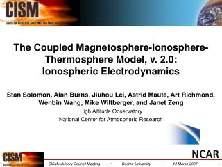
6. MIX - Electrodynamic Coupler • Uses the conservation of current to determine the cross polar cap potential • Computational domain • 2D slab of ionosphere, usually at 120 km altitude and from pole to 45 magnetic latitude • Calculates • Requires • FAC distribution • Plasma T and ρ to calculate energy flux of precipitating electrons • F107 or conductance Space Weather Workshop

7. Performance • CMIT Performance is a function of resolution in the magnetosphere ionosphere system • Low resolution • 53x24x32 cells in magnetosphere with variable resolution smallest cells ½ RE • 5° x 5° with 49 pressure levels in the ionosphere-thermosphere • On 8 processors of an IBM P6 it takes 20 minutes to simulate 1 hour • Modest resolution • 53x48x64 cells in the magnetosphere with variable resolution smallest cells ¼ RE • 2.5° x 2.5° with 98 pressure levels in the ionosphere-thermosphere • On 24 processors of an IBM P6 it takes an hour to simulate an hour Space Weather Workshop

8. Whole Heliosphere Interval • As part of IHY the WHI was chosen as a follow on to the WSM • Internationally coordinated observing and modeling effort to characterize solar-heliospheric-planetary system • Carrington Rotation 2068 • March 20 – April 16 2008 • Includes two high speed streams which are part of a co-rotating interaction region Space Weather Workshop

9. Different Stream Interactions • Geospace response to each stream had different characteristics • Stream 1had prompt rise of Φ while stream 2 had delayed reaction • Stream 1 had higher Φ for longer than stream 2 even though Vx was lower • BZ plays an important role in determine geoeffectiveness of streams Space Weather Workshop

10. Magnetopause Crossing Threat Scores • Using GOES magnetic field data it is possible to detect when the magnetopause is pressed inside geosynchronous orbit during southward IMF • This is a relatively rare event so TSS, MTSS and HSS are good choice • LFM performs better under these circumstances then empirical models Space Weather Workshop

11. Storm-time Geosync Magnetic Field • Geostationary fields are scientific metric, especially of interest during storms • Results for 25 September 1998 Event • Data set GOES magnetic field (black) • Baseline Model is T03 Storm (red) • Test Model is LFM (green) • Comparison shows that MHD model has much weaker ring current and tail current compared to Tsyganenko especially near midnight and at storm peak Work by Chia-Lin Huang Space Weather Workshop

12. The December 2006 “AGU Storm”  TEC from TIE-GCM D TEC from CMIT D TEC from GPS Space Weather Workshop

13. Field Alginged Current Structure • Comparison of Iridium FAC observations with various resolutions of the LFM simulation results • Results show better agreement with boundaries at higher resolution, but with greater magnitude • Iridium R1 1.3MA • LFM Low 3 1.5MA • LFM Low 2 0.8MA • LFM High 2 2.5MA Space Weather Workshop

14. Regional dB/dt tool Space Weather Workshop

15. dB/dT Analysis Space Weather Workshop

16. Conclusions • CMIT has the capability to perform in faster than real time mode for long durations with minimal supervision • Numerous parameters of interest can be derived from the basic physics parameters output by the model • It is not perfect, still have areas of improvement • Essential to define the right metrics to assess the value using this model adds to forecasts Space Weather Workshop

17. Backup Slides Space Weather Workshop

18. Threat Scores • Threat Score (Critical Success Index) • TS = CSI = hits/(hits+misses+false alarms) • Range 0 to 1 with 1 perfect and 0 no skill • How well did the forecast ‘yes’ events correspond to the observed ‘yes’ events? • Measures the fraction of observed and/or forecast events that were correctly predicted. • Can be thought of as accuracy when correct negatives are removed from consideration • True Skill Statistic (Hanssen and KuipersDiscriminant) • TSS = (hits)/(hits+misses) – (false alarms)/(false alarms+correctnegs) • Range -1 to 1 with 1 perfect and 0 no skill • How well did the forecast separate the ‘yes’ events from the ‘no’ events? • Can be thought of as POD - POFD • Uses all elements of the contingency table. • For rare events its unduly weighted toward the first term • Modifed True Skill Statistic • TSS2 = (hits-misses)/(hits+misses) – 2*(false alarms)/(correct negs) • Range -1 to 1 with 1 perfect and 0 no skill • First term is POD remapped to -1 to 1 • Second term peanlizes a forecast for large area for rare event Space Weather Workshop