Download
1 / 27
270 likes | 384 Vues
Gradients or hierarchies? Which assumptions make a better map?. Emilie B. Grossmann Janet L. Ohmann Matthew J. Gregory Heather K. May. How does the world work?. The World is a Gradient Curtis 1957 The Vegetation of Wisconsin The World is a Hierarchy Delcourt et al. 1983

E N D
Gradients or hierarchies? Which assumptions make a better map? Emilie B. Grossmann Janet L. Ohmann Matthew J. Gregory Heather K. May
How does the world work? • The World is a Gradient • Curtis 1957 • The Vegetation of Wisconsin • The World is a Hierarchy • Delcourt et al. 1983 • The World is Shaped by Many Different Things • Wimberly and Spies 2001 Influences of environment and disturbance on forest patterns in coastal Oregon watersheds • “No single theoretical framework was sufficient to explain the vegetation patterns observed in these forested watersheds.”
Tree Species Distributions Rainfall-Temperature Gradient Cool/Wet Hot/Dry Local Scale Regional Scale Forest Structure Canopy Closure Time Since Disturbance Short-term Long-term Regional-Scale Vegetation in Western Oregon:a (very) simple conceptual model.
Tree Species Distributions Rainfall-Temperature Gradient Cool/Wet Hot/Dry Local Scale Regional Scale Forest Structure Canopy Closure Time Since Disturbance Short-term Long-term Spatial Data Covering Regional Scales in Western Oregon Elevation Climate (PRISM) Soil Parent Material Local Topography LANDSAT (bands and transformations)
Our Quest • Make a highly accurate regional-scale vegetation map, that simultaneously represents detailed forest composition and structure.
Perils • Peril #1: • The world is a complex place. • Solution #1: • Use statistical models to sort out the complexity, and make a prediction. • Peril #2: • Statistical models often come with ASSUMPTIONS that cause problems when violated. • Solution #2: • Try to find a model with reasonable assumptions. • See whether it works any better than other methods.
Methods Maps built from: 1677 plots (FIA annual plots) 19 possible mapped explanatory variables.
Methods: k-NN (2) Place new pixel within feature space study area (4) impute nearest neighbor’s value to pixel (3) find nearest-neighbor plot within feature space feature space geographic space Elevation (1) Place plots within feature space Rainfall
Methods: GNN (2) calculate axis scores of pixel from mapped data layers study area (4) impute nearest neighbor’s value to pixel (3) find nearest-neighbor plot in gradient space ASSUMPTION: Species exhibit unimodal responses to environmental variables. gradient space geographic space CCA Axis 2 (e.g., Temperature, Elevation) (1) conduct gradient analysis of plot data CCA Axis 1 (e.g., Rainfall, local topography)
Methods: Random Forest Nearest Neighbor Imputation study area Random Forest space geographic space ?
Methods: Classification Tree Elevation < 1244 August Maximum < 25.60 Temp August Maximum < 23.24 Temp Summer Mean < 12.79 Temp Aug. to Dec. Temperature < 12.79 Differential LANDSAT Band 5 < 24 Elevation < 1625 PSME PIPO TSHE PSME ABAM TSME PSME THPL High Elevation ( > 1244) High August Temp (> 23.24°C) High reflectance in Band 5 (> 24)
Methods: Random Forest A “Forest” of classification trees. Each tree is built from a random subset of plots and variables.
Methods: Random Forest Imputation 28 29 26 16 20 28 30 27 26 2 3 6 10 1 5 7 9 15 8 14 13 11 18 19 25 24 23 17 16 20
Accuracy Assessment • Species Kappa • RMSD • Bray-Curtis Distance
Forest Structure: Basal Area k-NN GNN RFNN PERIL! COMPUTING TIME! Random forest took over a week to run. Just finished last Friday morning. If you are in a rush to prepare for a conference, don’t take this route!!!
Summary • Species Kappas • Each model had strengths and weaknesses. • All did well with the dominants. • Structure • RFNN consistently just a little bit better. • Maps • Broad-scale: Indistinguishable • Local-scale: GNN noisiest • Overall Community Structure • RFNN best.
Conclusion • Random forest did the best all around. broad-scale (species composition) AND local-scale (structure) But, there’s still room for improvement.