Download
1 / 55
550 likes | 631 Vues
02/10/11. Finding Edges and Straight Lines. Computer Vision CS 543 / ECE 549 University of Illinois Derek Hoiem. Many slides from Lana Lazebnik, Steve Seitz, David Forsyth, David Lowe, Fei-Fei Li. Last class. How to use filters for Matching Denoising Compression

E N D
02/10/11 Finding Edges and Straight Lines Computer Vision CS 543 / ECE 549 University of Illinois Derek Hoiem Many slides from Lana Lazebnik, Steve Seitz, David Forsyth, David Lowe, Fei-Fei Li
Last class • How to use filters for • Matching • Denoising • Compression • Image representation with pyramids • Texture and filter banks
A couple remaining questions from earlier • Does the curvature of the earth change the horizon location? Illustrations from Amin Sadeghi
A couple remaining questions from earlier • Computational complexity of coarse-to-fine search? Image 1 Pyramid Image 2 Pyramid Size M Size N Repeated Local Neighborhood Search O(M) Downsampling: O(N+M) Low Resolution Search O(N/M) Overall complexity: O(N+M) Original high-resolution full search: O(NM) or O(N logN)
A couple remaining questions from earlier • Why not use an ideal filter? Answer: has infinite spatial extent, clipping results in ringing Attempt to apply ideal filter in frequency domain
Today’s class • Detecting edges • Finding straight lines
Why do we care about edges? Vertical vanishing point (at infinity) Vanishing line Vanishing point Vanishing point • Extract information, recognize objects • Recover geometry and viewpoint
Origin of Edges • Edges are caused by a variety of factors surface normal discontinuity depth discontinuity surface color discontinuity illumination discontinuity Source: Steve Seitz
Characterizing edges intensity function(along horizontal scanline) first derivative edges correspond toextrema of derivative • An edge is a place of rapid change in the image intensity function image
With a little Gaussian noise Gradient
Effects of noise Where is the edge? • Consider a single row or column of the image • Plotting intensity as a function of position gives a signal Source: S. Seitz
Effects of noise • Difference filters respond strongly to noise • Image noise results in pixels that look very different from their neighbors • Generally, the larger the noise the stronger the response • What can we do about it? Source: D. Forsyth
Solution: smooth first g f * g • To find edges, look for peaks in f Source: S. Seitz
Derivative theorem of convolution f • Differentiation is convolution, and convolution is associative: • This saves us one operation: Source: S. Seitz
Derivative of Gaussian filter • Is this filter separable? * [1 -1] =
Tradeoff between smoothing and localization • Smoothed derivative removes noise, but blurs edge. Also finds edges at different “scales”. 1 pixel 3 pixels 7 pixels Source: D. Forsyth
Designing an edge detector • Criteria for a good edge detector: • Good detection: the optimal detector should find all real edges, ignoring noise or other artifacts • Good localization • the edges detected must be as close as possible to the true edges • the detector must return one point only for each true edge point • Cues of edge detection • Differences in color, intensity, or texture across the boundary • Continuity and closure • High-level knowledge Source: L. Fei-Fei
Canny edge detector • This is probably the most widely used edge detector in computer vision • Theoretical model: step-edges corrupted by additive Gaussian noise • Canny has shown that the first derivative of the Gaussian closely approximates the operator that optimizes the product of signal-to-noise ratio and localization J. Canny, A Computational Approach To Edge Detection, IEEE Trans. Pattern Analysis and Machine Intelligence, 8:679-714, 1986. Source: L. Fei-Fei
Example original image (Lena)
Derivative of Gaussian filter y-direction x-direction
Compute Gradients (DoG) X-Derivative of Gaussian Y-Derivative of Gaussian Gradient Magnitude
Get Orientation at Each Pixel • Threshold at minimum level • Get orientation theta = atan2(gy, gx)
Non-maximum suppression for each orientation At q, we have a maximum if the value is larger than those at both p and at r. Interpolate to get these values. Source: D. Forsyth
Hysteresis thresholding • Threshold at low/high levels to get weak/strong edge pixels • Do connected components, starting from strong edge pixels
Hysteresis thresholding • Check that maximum value of gradient value is sufficiently large • drop-outs? use hysteresis • use a high threshold to start edge curves and a low threshold to continue them. Source: S. Seitz
Canny edge detector • Filter image with x, y derivatives of Gaussian • Find magnitude and orientation of gradient • Non-maximum suppression: • Thin multi-pixel wide “ridges” down to single pixel width • Thresholding and linking (hysteresis): • Define two thresholds: low and high • Use the high threshold to start edge curves and the low threshold to continue them • MATLAB: edge(image, ‘canny’) Source: D. Lowe, L. Fei-Fei
Effect of (Gaussian kernel spread/size) original Canny with Canny with • The choice of depends on desired behavior • large detects large scale edges • small detects fine features Source: S. Seitz
Learning to detect boundaries • Berkeley segmentation database:http://www.eecs.berkeley.edu/Research/Projects/CS/vision/grouping/segbench/ human segmentation image gradient magnitude
pB boundary detector Martin, Fowlkes, Malik 2004: Learning to Detection Natural Boundaries… http://www.eecs.berkeley.edu/Research/Projects/CS/vision/grouping/papers/mfm-pami-boundary.pdf Figure from Fowlkes
pB Boundary Detector Figure from Fowlkes
Brightness Color Texture Combined Human
Finding straight lines • One solution: try many possible lines and see how many points each line passes through • Hough transform provides a fast way to do this
Outline of Hough Transform • Create a grid of parameter values • Each point votes for a set of parameters, incrementing those values in grid • Find maximum or local maxima in grid
Finding lines using Hough transform • Using m,b parameterization • Using r, theta parameterization • Using oriented gradients • Practical considerations • Bin size • Smoothing • Finding multiple lines • Finding line segments
3. Hough votes Edges Find peaks and post-process
Hough transform example http://ostatic.com/files/images/ss_hough.jpg
Finding circles using Hough transform • Fixed r • Variable r
Finding straight lines • Another solution: get connected components of pixels and check for straightness
Finding line segments using connected components • Compute canny edges • Compute: gx, gy (DoG in x,y directions) • Compute: theta = atan(gy / gx) • Assign each edge to one of 8 directions • For each direction d, get edgelets: • find connected components for edge pixels with directions in {d-1, d, d+1} • Compute straightness and theta of edgelets using eig of x,y 2nd moment matrix of their points • Threshold on straightness, store segment Larger eigenvector