Download
1 / 34
380 likes | 625 Vues
Closed Testing and the Partitioning Principle. Jason C. Hsu The Ohio State University MCP 2002 August 2002 Bethesda, Maryland. Principles of Test-Construction. Union-Intersection Testing UIT S. N. Roy Intersection-Union Testing IUT Roger Berger (1982) Technometrics Closed testing

E N D
Closed Testing and the Partitioning Principle Jason C. Hsu The Ohio State University MCP 2002August 2002Bethesda, Maryland
Principles of Test-Construction • Union-Intersection Testing UIT S. N. Roy • Intersection-Union Testing IUT Roger Berger (1982) Technometrics • Closed testing Marcus, Peritz, Gabriel (1976) Biometrika • Partitioning Stefansson, Kim, and Hsu (1984) Statistical Decision Theory and Related Topics, Berger & Gupta eds., Springer-Verlag. Finner and Strassberger (2002)Annals of Statistics • Equivariant confidence set Tukey (1953) Scheffe (195?) Dunnett (1955)
Partitioning confidence sets • Multiple Comparison with the Best Gunnar Stefansson & Hsu • 1-sided stepdown method (sample-determined steps) = Naik/Marcus-Peritz-Gabriel closed test Hsu • Multiple Comparison with the Sample Best Woochul Kim & Hsu & Stefansson • Bioequivalence Ruberg & Hsu & G. Hwang & Liu & Casella & Brown • 1-sided stepdown method (pre-determined steps) Roger Berger & Hsu
Partitioning • Formulate hypotheses H0i: i* for iI • iIi* = entire parameter space • {i*: iI} partitions the parameter space • Test each H0i*: i *, iI, at • Infer i if H0i* is rejected • Pivot in each i a confidence set Ci for • iICi is a 100(1)% confidence set for
Partitioning • Formulate hypotheses H0i: i for i I • iJ I = entire parameter space • For each J I, letJ * = iJi( jJj)c • Test each H0J*: J *, J I, at • {J*: J I} partitions the parameter space • Infer J if H0J* is rejected • Pivot in each J a confidence set CJ for • J J CJ is a 100(1)% confidence set for
MCB confidence intervals i maxji j [(Yi maxji Yj W), (Yi maxji Yj+ W)+], i = 1, 2, … , k • Upper bounds imply subset selection • Lower bounds imply indifference zone selection
Multiple Comparison with the Best • H01: Treatment 1 is the best • H02: Treatment 2 is the best • H03: Treatment 3 is the best • … • Test each at using 1-sided Dunnett’s • Collate the results
Union-Intersection Testing UIT • Form Ha: Hai(an “or” thing) • Test H0: H0i, the complement of Ha • If reject, infer at least one H0i false • Else, infer nothing
Closed Testing • Formulate hypotheses H0i: i for iI • For each JI, let J = iJi • Form closed family of null hypotheses{H0J: J: JI} • Test each H0J at • Infer iJi if all H0J’ with J J’ rejected • Infer i if all H0J’ with i J’ rejected
Oneway model Yir = i + ir, i = 0, 1, 2, … , k, r = 1, … , ni ir are i.i.d. Normal(0, 2) Dose i “efficacious” if i > 1 + ICH E10 (2000) • Superiority if 0 • Non-inferiority if < 0 • Equivalence is 2-sided • Non-inferiority is 1-sided
Closed testing null hypotheses(sample-determined steps) • H02: Dose 2 not efficacious • H03: Dose 3 not efficacious • H01: Doses 2 and 3 not efficacious • Test each at • Collate the results
Partitioning null hypotheses(sample-determined steps) • H01: Doses 2 and 3 not efficacious • H02: Dose 2 not efficaciousbut dose 3 is • H03: Dose 3 not efficaciousbut dose 2 is • Test each at • Collate the results
Partitioning implies closed testing Partitioning implies closed testing because • A size test for H0i is a size test forH0i • Reject H01: Doses 2 and 3 not efficacious implies either dose 2 or dose 3 efficacious • Reject H02: Dose 2 not efficaciousbut dose 3 efficacious implies it is not the case dose 3 is efficacious but notdose 2 • Reject H01 and H02 thus implies dose 2 efficacious
Intersection-Union Testing IUT • Form Ha: Hai (an “and” thing) • Test H0: H0i, the complement of Ha • If reject, infer all H0i false • Else, infer nothing
Bioequivalence defined Bioequivalence: clinical equivalence between • Brand name drug • Generic drug Bioequivalence parameters • AUC = Area Under the Curve • Cmax = maximum Concentration • Tmax = Time to maximum concentratin
Average bioequivalence Notation = expected value of brand name drug 2 = expected value of generic drug Average bioequivalence means .8 < /2 < 1.25 for AUC and .8 < /2 < 1.25 for Cmax
Bioequivalence in practice If log of observations are normal with means and2 and equal variances, then average bioequivalence becomes log(.8) < 2 < log(1.25) for AUC and log(.8) < 2 < log(1.25) for Cmax
Partitioning Partition the parameter space as • H0<: 2 < log(0.8) • H0>: 2 > log(1.25) • Ha: log(.8) < 2 < log(1.25) Test H0< and H0> each at . Infer log(.8) < 2 < log(1.25) if both H0< and H0> rejected. Controls P{incorrect decision} at .
Anti-psychotic drug efficacy trial Arvanitis et al. (1997 Biological Psychiatry) CGI = Clinical Global Impression
Minimum Effective Dose (MED) Minimu Effective Dose = MED = smallest i so that i > 1 + for all j, i j k Want an upper confidence bound MED+so that P{MED < MED+} 100(1)%
Closed testing inference • Infer nothing if H01 is accepted • Infer at least one of doses 2 and 3 effective if H01 is rejected • Infer dose 2 effective if, in addition to H01,H02 is rejected • Infer dose 3 effective if, in addition to H01,H03 is rejected
Closed testing method(sample-determined steps) • Start from H01 to H02 and H03 • Stepdown from smallest p-value to largest p-value • Stop as soon as one fails to reject • Multiplicity adjustment decreases from k to k 1 to k 2 to 2 from step 1 to 2 to 3 … to step k 1
Tests of equalities(pre-determined steps) • H0k: 1 = 2 = = kHak: 1 = 2 = < k • H0(k1): 1 = 2 = = k1Ha(k1): 1 = 2 = < k1 • H0(k2): 1 = 2 = = k2Ha(k2): 1 = 2 = < k2 • • H02: 1 = 2Ha2: 1 < 2
Closed testing of equalities • Null hypotheses are nested • Closure of family remains H0k H02 • Test each H0i at • Stepdown from dose k to dose k1 to to dose 2 • Stop as soon as one fails to reject • Multiplicity adjustment not needed
H0k: 1 = = k H02: 1 = 2 H0i H0i H0k: 1 k H02:1 2 H0i H0i Testing equalities is easy
Partitioning null hypotheses (for pre-determined steps) • H0k: Dose k not efficacious • H0(k-1):Dose k efficacious but dose k1 not efficacious • H0(k-1):Doses k and k1 efficacious but dose k2 not efficacious • • H02: Doses k 3 efficacious but dose 2 not efficacious • Test each at • Collate the results
Partitioning inference • Infer nothing if H0k is accepted • Infer dose k effective if H0k is rejected • Infer dose k1 effective if, in addition to H0k, H0(k-1) is rejected • Infer dose k2 effective if, in addition to H0k and H0(k-1) , H03 is rejected •
Partitioning method (for pre-determined steps) • Stepdown from dose k to dose k1 to to dose 2 • Stop as soon as one fails to reject • Multiplicity adjustment not needed • Any pre-determined sequence of doses can be used • Confidence set given in Hsu and Berger (1999 JASA)
Pairwise t tests for partitioning Size tests for H0k H02 are also size test forH0k H02 • H0k: Dose k not efficacious • H0(k-1): Dose k1 not efficacious • H0(k-2): Dose k2 not efficacious • • H02: Dose 2 not efficacious • Test each with a size- 2-sample 1-sided t-test
H0k: 1 = = k H02: 1 = 2 H0i H0i H0k: 1 k H02:1 2 H0i H0i Testing equalities is easy
Could reject for the wrong reason H0 Ha neither