Download
1 / 34
340 likes | 525 Vues
Spatiotemporal Saliency Map of a Video Sequence in FPGA hardware. David Boland Acknowledgements: Professor Peter Cheung Mr Yang Liu. What is Spatiotemporal Saliency?. Saliency – parts of a scene that appear pronounced

E N D
Spatiotemporal Saliency Map of a Video Sequence in FPGA hardware David Boland Acknowledgements: Professor Peter Cheung Mr Yang Liu
What is Spatiotemporal Saliency? • Saliency – parts of a scene that appear pronounced • Spatiotemporal Saliency – parts of a scene that appear pronounced in video
Why Important? • General environments are complex and dynamic • Human eye handles this by focusing upon salient objects • Real-time algorithm to emulate this has many uses: • Image processing • Surveillance • Machine vision • Navigation…
The Problem • Spatiotemporal Saliency algorithms have high computational complexity. • Store stack of video frames • Unsuitable for real-time • Need algorithm with reduced memory requirements
Overview • Introduce Algorithm and section completed • Brief background • Implementation • Software Model • Hardware Model • Results • Optimisations (if time) • Summary
Feature Tracking Module • Object tracking generally achieved through monitoring optical flow • Optical flow: “the distribution of apparent velocities of movement of brightness patterns in an image” • Several Algorithms – None perfect • Good Trade complexity vs. accuracy – Lukas Kanade Algorithm
Lukas Kanade Algorithm • Definition of problem: • Let I and J are two consecutive images • Let u = [ux, uy ] be an image point in I • Find v = u + d = [ux+dx, uy+dy] where v is a similar point on J • Points not tracked equally due to aperture problem. • Solution is to minimise error:
Lukas Kanade Solution (Iteratively Refine) Find where
Pyramidal Lukas Kanade Algorithm • Lukas Kanade Algorithm assumes small motion • Handle Larger motion with window size • But Lose Accuracy • Solution • Create Hierarchy of images • Each image ½ as large • Perform Lukas Kanade on each level to get guess • Map guess to lower levels
Pyramidal Lukas Kanade Algorithm Map guess to lower levels, obtain better guess Find final pixel location Track feature between two images at the highest level to obtain guess for new feature location Apply LK, start at guess Apply LK, start at guess Apply LK
Implementation – Software Model • Why? • Results to test the hardware against • Useful during debugging stage • Choice of Software Language: Matlab • Matrix calculations • Maps well to hardware • Simple for fast development • Method: • Apply feature detection algorithm to find co-ordinates • Apply Pyramidal Lukas Kanade to track co-ordinates
Implementation – Hardware • Aims: • Fit onto the FPGA • Clock Frequency 65MHz for VGA • Not Straightforward: • Initial design emulate software correctly: • Well over 200% size of FPGA • Initial Design 4MHz
Hardware Considerations • Choice Software Language: Handel-C • Minimise expensive operations • Memory Accesses • Multiplication • Division • Maintain Precision • Floating point precision unavailable • General Optimisations • Minimise Delay Path or Logic Depth • Minimise Fan-out
Memory Considerations – Building Hierarchy • To build image of higher level: • Iterate over even pixels • Collect mask of values surrounding the pixel • Weight as shown on right • Sum • Repeat recursively on output for higher levels
Memory Considerations – Building Hierarchy • Pixels re-used: • Store locally • Reduce Memory reads
Memory Considerations – Optical Flow • Only read once values once from main memory • Also reduce fan-out
Multiplications • Avoid via left-shifting • Pre-compute results whenever possible • Use Dedicated Multipliers • Combined for large multiplications
Division Considerations • Division Costly process • Handel-C designs hardware to implement in one cycle. • Large number of bits implies large delay • Solution: Spread over multiple cycles • Long Division • Slow – unbounded stage • Binary Search • If limit range of optical flow per iteration [-1 1]
1 B ≥ ≥ 0.825B < 0.75 B 0.75 B ≥ ≥ < 0.625B < 0.5 B 0.5 B ≥ 0.375 B ≥ < < 0.25 B 0.25 B ≥ < 0.125B < 0 B Division Considerations A/B=x ≡ A=B*x
Division Considerations 1 B 111 1 0.825B 1 0 0.75 B 0.75 B 110/101 1 1 0 0.625B 0 0.5 B 0.5 B 100/011 1 0.375B 1 0 0 0.25 B 0.25 B 010/001 1 0 0.125B 0 0 B 000
Hardware Testing • Test against software model • Store Feature co-ordinates & tracked locations from software model • Load feature co-ordinates in hardware • Track in hardware • Compare difference • Vary number of fractional bits • Examine importance/cost of different fractional precision
Results Summary • Final design only uses 1/6 FPGA • Use 4/5/6 fractional bits for good accuracy • Speed short of desired (approx 50 MHz) • ISE estimates cautious • Pipelining can increase this • Reduced Loop control
Optimisations • Final Design only uses 1/6 FPGA. • Use space to increase Speed: • Pipelined Hardware • Parallel Hardware
Summary • Spatiotemporal Saliency framework • Role of optical flow within framework • Steps to create & test hardware implementation • Effective method to find optical flow • High Speed/Accuracy, small area • Optimisations to achieve this • Further Improvements possible • Some performance advantages over other hardware optical flow implementations • Optical flow useful beyond Spatiotemporal Saliency Framework