Download
1 / 33
340 likes | 531 Vues
A bottom up visual saliency map in the primary visual cortex --- theory and its experimental tests. Li Zhaoping. University College London. Invited presentation at COSYNE (computational and systems Neuroscience) conference Salt Lake City, Utah, Feb. 2007. Test 1:.

E N D
A bottom up visual saliency map in the primary visual cortex --- theory and its experimental tests. Li Zhaoping University College London Invited presentation at COSYNE (computational and systems Neuroscience) conference Salt Lake City, Utah, Feb. 2007.
Test 1: V1 explains the known behavoral data on visual saliency Test 2: Psychophysical tests of the predictions of the V1 theory on previously unknown visual selection behavior. Outline Saliency --- for visual selection and visual attention Hypothesis --- of a saliency map in the primary visual cortex ( V1) theory
Visual selection Top-down selection: goal directed Bottom-up selection: input stimulus driven Focus of this talk Attentional bottle neck Visual inputs Visual Cognition Selected information 40 bits/second (Sziklai 1956) Many megabytes per second (Desimone & Duncan 1995, Treisman (1980), Tsotsos (1991), Duncan & Humphreys (1989), etc.) Faster and more potent (Jonides 1981, Nakayama & Mackeben 1989)
Bottom up visual selection and visual saliency Studied in visual search Feature search (Treisman & Gelade 1980, Julesz 1981, Wolfe et al 1989, Duncan & Humphreys 1989 etc) Reaction time (RT) Conjunction search # of distractors Unique conjunction of red color and vertical orientation Visual inputs The vertical bar pops out --- very fast, parallel, pre-attentive, effortless. slow & effortful
Bottom up visual selection and visual saliency Saliency map Visual inputs To guide attentional selection. (Koch & Ullman 1985, Wolfe et al 1989, Itti & Koch 2000, etc.) Question: where is the saliency map in the brain? Hint: selection must be very fast, the map must have sufficient spatial resolution
Hypothesis: The primary visual cortex (V1) creates a saliency map (Li, Z . Trends in Cognitive Sciences, 2002) Higher visual areas for other functions V1 neural firing rates Retina inputs Superior Colliculus to drive gaze shift Neural activities as universal currency to bid for visual selection. The receptive field of the most active V1 cells is selected How does V1 do it? (explained in a moment)
1 $pike 3 $pike A motion tuned V1 cell A color tuned V1 cell Attention auctioned here, no discrimination between your feature preferences, only spikes count! Hmm… I am feature blind anyway Attention does not have a fixed price! Capitalist… he only cares about money!!! auctioneer 2 $pike An orientation tuned V1 cell Zhaoping L. 2006, Network: computation in neural systems
Questions one may ask(answered in Zhaoping 2006, network, or ask me after the talk) Haven’t the others said that V1 is only a low-level area, and the saliency map is in LIP (Gottlieb & Goldberg 1998), FEF, or higher cortical areas? --- short answer, “yes” Didn’t you say more than a decade ago that V1 does efficient (sparse) coding which also serves object invariance? --- short answer, “yes” Do you mean that cortical areas beyond V1 could not contribute to saliency additionally? --- short answer “no”. Do you mean that V1 does not also play a role in learning, object recognition, and other goals? --- short answer “no”
How does V1 do it ? (after all saliency depends on context) Cells tuned to orientation, color, or both can all respond to a single item Saliency map Maximum response at each location V1 Intra-cortical interactions in V1 make nearby neurons tuned to the similar features suppress each other --- iso-feature suppression (Gilbert & Wiesel 1983, Rockland & Lund 1983, Allman et al 1985, Hirsch & Gilbert 1991, etc) Visual input
Physiologically observed in V1: Contextual influences(since 1970s, Allman et al 1985, Knierim van Essen 1992, Hirsch & Gilbert 1991, Kapadia et al 1995, Nothdurft et al 1999 etc) Strong suppression Weak suppression suppression facilitation 18 spikes/s 10 spikes/s 5 spikes/s Dominant Classical receptive fields Hubel & Wiesel 1962 Single bar e.g., 20 spikes/s
Testing the V1 saliency map --- 1 ‘+’ among ‘|’s --- easy Feature search --- easy Few physiological data difficult experiments …. ‘|’ among ‘+’s --- difficult Conjunction search --- difficult ‘ ‘ among ‘ ‘s regular background ---difficult ‘ ‘ among ‘ ‘s irregular background ---difficult Explain V1 outputs Saliencies in visual search and segmentation Solution: build a V1 model multi-unit recording on the model (Li, 1998, 1999, 2000, 2002, etc) More examples in literature, e.g., Treisman & Gelade 1980, Julesz 1981, Duncan & Humphreys 1989, Wolfe et al 1989, etc.
Implementing the saliency map in a V1 model Saliency output from V1 model Highlighting important image locations, where translation invariance in inputs breaks down. A recurrent network with Intra-cortical Interactions that executes contextual influences Contrast input to V1 V1 outputs V1 model
Schematics of how the model works V1 outputs Recurrent connection pattern Intra-cortical interactions V1 units and initial responses Sampled by the receptive fields Original image Designed such that the model agrees with physiology results on contextual influences.
Recurrent connections Intra-cortical Interactions Input , after filtering through classical receptive fields Recurrent dynamics -- differential equations of firing rate neurons interacting with each other with sigmoid like nonlinearity. See Li (1998, 1999, 2001), Li & Dayan (1999) for the mathematical analysis and computational design of the nonlinear dynamic. Output V1 model
Constraints used to design the intra-cortical interactions. Outputs Inputs Highlight boundary Enhance contour No symmetry breaking (hallucination) No gross extension Design techniques: mean field analysis, stability analysis. Computation desired constraints the network architecture, connections, and dynamics. Network oscillation and synchrony between neurons to the same contour is one of the dynamic consequences (Li, 2001, Neural Computation).
Make sure that the model can reproduce the usual physiologically observed contextual influences Iso-orientation suppression Random surround less suppression Cross orientation least suppression Co-linear facilitation Single bar Input output
Multi-unit recording on the model to view the saliency map Saliency map S=0.2, maximum firing rate at each location S=0.4, S=0.12, S=0.22 Pop-out Histogram of all responses S regardless of features Z=7 s Z = (S-S)/σ --- z score, measuring saliencies of items σ Original input V1 response S
The V1 saliency map agrees with visual search behavior. input V1 model output Z=7 Target= Z= - 0.9 Feature search --- pop out Target = ‘+’ Conjunction search --- serial search
Explains a trivial example of search asymmetry V1 model output Z=7 Z=0.8 input Feature search --- pop out Target = + Target lacking a feature Target =
Explains background regularity effect V1 outputs Z=3.4 Z=0.22 Target= Inputs Homogeneous background, Target= Irregular distractor positions
More severe test of the saliency map theory by using subtler saliency phenomena --- search asymmetries (Treisman and Gormican 1988) Open vs. closed parallel vs. divergent long vs. short curved vs. straight ellipse vs. circle Z=0.41 Z= -1.4 Z= -0.06 Z= 0.3 Z= 0.7 Z=9.7 Z= 2.8 Z= 1.8 Z= 1.07 Z= 1.12
V1’s saliency computation on other visual stimuli V1 model output The smooth contours and the texture borders are the most salient Visual input Smooth contours in noisy background Texture segmentation --- simple textures Texture segmentation --- complex textures
input V1 output e.g., The cross is salient due to the horizontal bar alone --- the less salient vertical bar is invisible to saliency Predicting previously unknown behavior: psychophysical test Testing the V1 saliency map --- 2 Theory statement: the strongest response at a location signals saliency. Prediction: A task becomes difficult when the most salient feature is task irrelevant.
Test stimuli Prediction: segmenting this composite texture is much more difficult Note: if saliency at each location is determined by the sum of neural activities at each location, the prediction would not hold.
Task: subject answer whether the texture border is left or right Test: measure reaction times for segmentation:
Test: measure reaction times in the segmentation task: (Zhaoping and May, in press in PLoS Computational Biology, 2007) Reaction time (ms) Supporting V1 theory prediction !
Previous views on saliency map(since decades ago --- Koch & Ullman 1985, Wolfe et al 1989, Itti & Koch 2000 etc) Not in V1 Color feature maps orientation feature maps Other: motion, depth, etc. green Feature maps in V2, V3, V4, V? blue red green blue + Master saliency map in which cortical area? Visual stimuli
Previous views on saliency map(since decades ago --- Koch & Ullman 1985, Wolfe et al 1989, Itti & Koch 2000 etc) Visual stimuli motion, depth, etc. Color feature maps orientation Does not predict our data Feature maps blue + Master saliency map
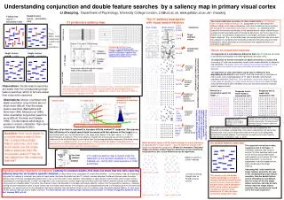
Colour pop out Orientation pop out Double feature pop out as in a race model double-feature advantage V1 theory prediction 2: --- double-feature advantage RT = 500 ms RT = 600 ms RT = ? RT = 500 ms or RT< 500 ms
Colour pop out Orientation pop out Double feature pop out RT <= 500 ms double-feature advantage on average V1 theory prediction 2: --- double-feature advantage Color tuned cell dictates saliency RT = 500 ms Orientation tuned cell dictates saliency RT = 600 ms Color, or, Orientation, or Color +Orientation conjunctive tuned cell dictates saliency RT = ? RT = 500 ms or RT< 500 ms
RT V1 saliency Prediction --- double- feature advantage for C+O, O+M, but not C+M Race model prediction Fingerprint of V1:It is known that V2 has cells tuned to all types of conjunctive cells, including C+M (Gegenfurtner et al 1996). C+O O+MC+M RT Race model prediction If V2 or higher cortical areasare responsible for saliency --- double-feature advantage forC+O, O+M and C+M. C+O O+MC+M V1 theory prediction 2: --- double-feature advantage In V1, conjunctive cells exist for C+O, O+M, but not for C+M (Livingstone & Hubel 1984, Horwitz & Albright 2005)
V1 theory prediction 2: --- double-feature advantage for C+O, O+M, but not for C+M Test:compare the RT for double-feature search with that predicted by the race model (Koene & Zhaoping ECVP 2006) Normalized RT for 7 subjects Race model prediction Confirming V1’s fingerprint C+O O+M C+M
Summary:A theory of a bottom up saliency map in V1 Tested by (1)V1 outputs accounts for previous saliency data • (2) New data confirms theory’s predictions The theory links physiology with behavior, And challenges the previous views about the role of V1 and about the psychophysical saliency map. Since top-down attention has to work with or against the bottom up saliency, V1 as the bottom up saliency map has important implications about top-down attentional mechanisms.