Download
1 / 40
430 likes | 676 Vues
Saliency-baesd Visual Attention. 黃文中 2009-01-08. Outline. Introduction The Model Results Conclusion. Outline. Introduction The Model Results Conclusion. If we are asking to find…. Where to look?. Many visual processes are expensive Humans don’t process the whole visual field

E N D
Saliency-baesd Visual Attention 黃文中 2009-01-08
Outline • Introduction • The Model • Results • Conclusion
Outline • Introduction • The Model • Results • Conclusion
Where to look? • Many visual processes are expensive • Humans don’t process the whole visual field • How do we decide what to process? • How can we use insights about this to make machine vision more efficient?
Visual salience • Salience ~ visual prominence • Must be cheap to calculate • Related to features that we collect from very early stages of visual processing • Colour, orientation, intensity change and motion are all important indicators of salience
Saliency Map • The Saliency Map is a topographically arranged map that represents visual saliency of a corresponding visual scene.
Saliency map (Cont'd) • Two kinds of stimuli type: • Bottom-up • Depend only on the instantaneous sensory input • Without taking into account the internal state of the organism • Top-down • Take into account the internal state • Such as goals the organisms has at this time, personal history and experiences, etc
Outline • Introduction • The Model • Results • Conclusion
Three main step • Extraction • extract feature vectors at locations over the image plane • Activation • form an "activation map" (or maps) using the feature vectors • Normalization / Combination • normalize the activation map (or maps, followed by a combination of the maps into a single map)
In detail… • Nine spatial scales are created using dyadic Gaussian pyramids. • Each features is computed by a set of linear “center-surround” operations akin to visual receptive fields. • Normalization • Across-scale combination into three “conspicuity maps.” • Linear combinations to create saliency map. • Winner-take-all
Image pyramids • The original image is decomposed into sets of lowpass and bandpass components via Gaussian and Laplacian pyramids. • The Gaussian pyramid consists of lowpass filtered (LPF). • The Laplacian pyramid consists of bandpass filtered (BPF).
Extraction of early visual features • Intensity image: • Color channels: • Local orientation information: Obtained from using oriented Gabor pyramids
In detail… • Nine spatial scales are created using dyadic Gaussian pyramids. • Each features is computed by a set of linear “center-surround” operations akin to visual receptive fields. • Normalization • Across-scale combination into three “conspicuity maps.” • Linear combinations to create saliency map. • Winner-take-all
Center-surround differences • is obtained by interpolation to the finer scale and point-by-point substraction. • Intensity contrast: • Color double-opponent: • Orientation feature maps:
In detail… • Nine spatial scales are created using dyadic Gaussian pyramids. • Each features is computed by a set of linear “center-surround” operations akin to visual receptive fields. • Normalization • Across-scale combination into three “conspicuity maps.” • Linear combinations to create saliency map. • Winner-take-all
Map normalization operator • Map normalization operator:
Map normalization operator (Cont'd) • Normalizing the values in the map to a fixed range [0..M], in order to eliminate modality-dependent amplitude differences • Finding the location of the map’s global maximum M and computing the average m of all its other local maxima • Globally multiplying the map by .
Map normalization operator (Cont'd) • The method is called the global non-linear normalization. • Pros: • Computationally very simple. • Easily allows for real-time implementation because it is non-iterative. • Cons: • This strategy is not very biologically plausible, since global computations are used. • Not robust to noise, when noise can be stronger than the signal.
Iterative localized interactions • Non-classical surround inhibition • Interactions within each individual feature map rather than between maps • Inhibition appears strongest at a particular distance from the center, and weakens both with shorter and longer distances. • The structure of non-classical interactions can be coarsely modeled by a two-dimensional difference-of-Gaussians(DoG) connection pattern.
In detail… • Nine spatial scales are created using dyadic Gaussian pyramids. • Each features is computed by a set of linear “center-surround” operations akin to visual receptive fields. • Normalization • Across-scale combination into three “conspicuity maps.” • Linear combinations to create saliency map. • Winner-take-all
Across-scale combination • “ ”, which consists of reduction of each map to scale 4 and point-by-point addition:
In detail… • Nine spatial scales are created using dyadic Gaussian pyramids. • Each features is computed by a set of linear “center-surround” operations akin to visual receptive fields. • Normalization • Across-scale combination into three “conspicuity maps.” • Linear combinations to create saliency map. • Winner-take-all
The Saliency Map (SM) • The three conspicuity maps are normalized and summed into the final input S to the saliency map: • The weights of each channel is tunable.
In detail… • Nine spatial scales are created using dyadic Gaussian pyramids. • Each features is computed by a set of linear “center-surround” operations akin to visual receptive fields. • Normalization • Across-scale combination into three “conspicuity maps.” • Linear combinations to create saliency map. • Winner-take-all
Winner-take-all • At any given time, only one location is selected from the early representation and copied into the central representation.
Winner-take-all (Cont'd) • The FOA is shifted to the location of the winner neuron. • The global inhibition of the WTA is triggered and completely inhibits (resets) all WTA neurons. • Local inhibition is transiently activated in the SM, in an area with the size and new location of the FOA.
Outline • Introduction • The Model • Results • Conclusion
Model performance on noisy versions of pop-out and conjuctive tasks
Outline • Introduction • The Model • Results • Conclusion
Conclusion • Have proposed a conceptually simple computational model for saliency-driven focal visual attention. • The framework can consequently be easily tailored to arbitrary tasks through the implementation of dedicated feature maps.
References • L. Itti, C. Koch, E. Niebur, “A Model of Saliency-Based Visual Attention for Rapid Scene Analysis”, IEEE Transactions on Pattern Analysis and Machine Intelligence, Vol. 20, No. 11, pp. 1254-1259, Nov 1998. • L. Itti, C. Koch, A saliency-based search mechanism for overt and covert shifts of visual attention, Vision Research, Vol. 40, No. 10-12, pp. 1489-1506, May 2000. • H. Greenspan, S. Belongie, R. Goodman, P. Perona, S. Rakshit, and C.H. Anderson, “Overcomplete Steerable Pyramid Filters and Rotation Invariance,” Proc. IEEE Computer Vision and Pattern Recognition, pp. 222-228, Seattle, Wash., June 1994.