Download
1 / 14
140 likes | 277 Vues
Reflecting Policy Limits in the FFT Algorithm. James C. Sandor, FCAS, MAAA American Re-Insurance 2003 CAS Seminar on Reinsurance. Agenda. BRIEFLY review FFT algorithm Describe modification to reflect policy limits An example The algorithm in practice Questions. A Brief Review.

E N D
Reflecting Policy Limits in the FFT Algorithm James C. Sandor, FCAS, MAAA American Re-Insurance 2003 CAS Seminar on Reinsurance
Agenda • BRIEFLY review FFT algorithm • Describe modification to reflect policy limits • An example • The algorithm in practice • Questions
A Brief Review • Fast Fourier Transform (FFT) Algorithm • Collective Risk Model • Frequency/Severity Assumptions • Uses the Following Relationship • φZ(t) = PN(φX(t)) • φX is the characteristic function of the severity • PNis the PGF of the frequency • If we know these, we can calculate the characteristic function of the aggregate distribution, φZ(t) • FFT produces approximation of φX • IFFT gets us fz(z) from φZ
A Couple Details • The PGFsfor many common frequency distributions can be found in Loss Models • The severity must be discretized before we can use the FFT to get the characteristic function • Insert favorite method here (rounding, mean-preserving, etc.)
Basic Assumptions Underlying Method • Collective Risk Model • One frequency distribution • One severity distribution • Assumes layer is fully exposed • Layer can be ground-up
Modification • Still one severity distribution • Weighted average of severity distributions at different limits • Weighted by underlying expected frequency
Practical Details • Assumptions • Expected Aggregate Loss • aka the 1st moment of the Aggregate Distribution • Severity Distribution • Frequency Moments relationship • Variance to Mean ratio
Practical Details • Expected Total Loss& • Severity Distribution • Expected Frequency(Both Ground-Up and Layer)Policy Limit Weights = Ground-Up Expected Frequency
An Example Severity Curve: ISO Commercial Auto Light/Medium (SG II)
Severity Distribution • Discretize Severity Distribution(s) • One distribution for each Policy Limit • Unconditional Layer Severities • If Retention > 0 then P(X=0)>0 • Distributions reflect Policy Limit and Layer • Final severity distribution = Weighted average of Individual Severities • Weights are Ground-up frequency
An Example Layer is 750,000 xs 250,000
Why is this correct? • Takes into account probability of hitting policy • Assumes Probability of hitting policy Expected Frequency • Assumes size of loss and policy limit are independent • That assumption can be easily modified • Use different severity for each limit
Finishing Up • Weighted average severity used as input into FFT algorithm • Taking into account policy limits can have a non-trivial impact on the Aggregate distribution
More Examples • Aggregate Modeling tool in Excel/MATLAB • Stochastic Reinsurance Pricing Model • Also in Excel/MATLAB