Download
1 / 10
100 likes | 225 Vues
Curve fit. noise= randn (1,30); x=1:1:30; y= x+noise 3.908 2.825 4.379 2.942 4.5314 5.7275 8.098 …………………………………25.84 27.47 27.00 30.96 [ p,s ]= polyfit (x,y,1); yfit = polyval ( p,x ); plot (x,y,'+',x,x,'r',x, yfit ,'b').

E N D
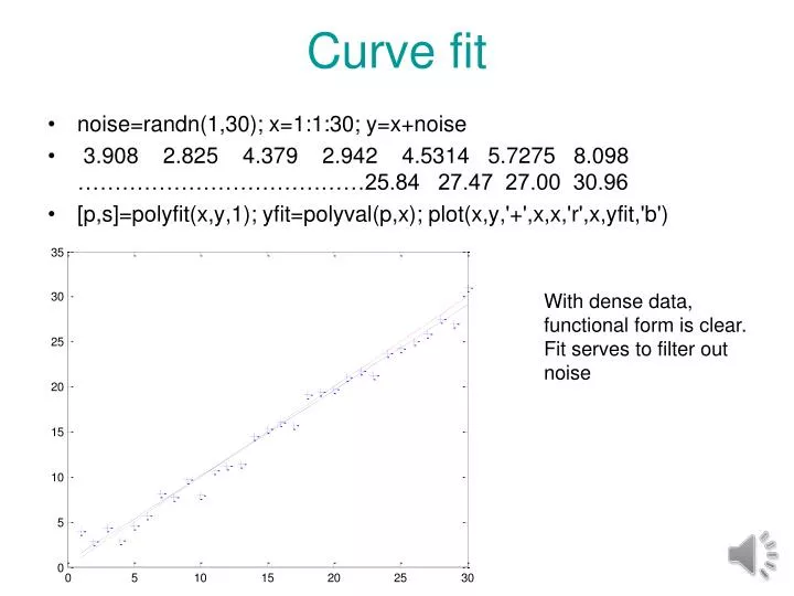
Curve fit • noise=randn(1,30); x=1:1:30; y=x+noise • 3.908 2.825 4.379 2.942 4.5314 5.7275 8.098 …………………………………25.84 27.47 27.00 30.96 • [p,s]=polyfit(x,y,1); yfit=polyval(p,x); plot(x,y,'+',x,x,'r',x,yfit,'b') With dense data, functional form is clear. Fit serves to filter out noise
Regression • The process of fitting data with a curve by minimizing root mean square error is known as regression • Term originated from first paper to use regression “regression of heights to the mean” http://www.jcu.edu.au/cgc/RegMean.html • Can get the same curve from a lot of data or very little. So confidence in fit is major concern.
Surrogate (approximations) • Originated from experimental optimization where measurements are very noisy • In the 1920s it was used to maximize crop yields by changing inputs such as water and fertilizer • With a lot of data, can use curve fit to filter out noise • “Approximation” can be then more accurate than data! • The term “surrogate” captures the purpose of the fit: using it instead of the data for prediction. • Most important when data is expensive
Surrogates for Simulation based optimization • Great interest now in applying these techniques to computer simulations • Computer simulations are also subject to noise (numerical) • However, simulations are exactly repeatable, and if noise is small may be viewed as exact. • Some surrogates (e.g. polynomial response surfaces) cater mostly to noisy data. Some (e.g. Kriging) to exact data.
Polynomial response surface approximations • Data is assumed to be “contaminated” with normally distributed error of zero mean and standard deviation • Response surface approximation has no bias error, and by having more points than polynomial coefficients it filters out some of the noise. • Consequently, approximation may be more accurate than data
Fitting approximation to given data • Noisy response model • Data from ny experiments • Linear approximation • Rational approximation • Error measures
Linear Regression • Functional form • For linear approximation • Estimate of coefficient vector denoted as b • Rms error • Minimize rms error eTe=(y-XbT)T(y-XbT) • Differentiate to obtain Beware of ill-conditioning!
Example 3.1.1 • Data: y(0)=0, y(1)=1, y(2)=0 • Fit linear polynomial y=b0+b1x • Then • Obtain b0=1/3, b1=0.
Comparison with alternate fits • Errors for regression fit • To minimize maximum error obviously y=0.5. Then eav=erms=emax=0.5 • To minimize average error, y=0 eav=1/3, emax=1, erms=0.577 • What should be the order of the progression from low to high?