An approach for the S-curve fit

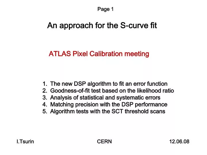
1. Page 1 An approach for the S-curve fit ATLAS Pixel Calibration meeting • The new DSP algorithm to fit an error function • Goodness-of-fit test based on the likelihood ratio • Analysis of statistical and systematic errors • Matching precision with the DSP performance • Algorithm tests with the SCT threshold scans I.Tsurin CERN 12.06.08

2. A couple of reasons for improvements 32 bits for 8-bit integers (unstable fits otherwise): Commissioning results: shown are the number of modules with more than 0.2% of pixels failing the online (DSP) fits Unstable offline results: (often mentioned) Page 2

3. ATLAS Pixel Threshold Scans Pixel parameters: signal gain, noise, time response are measured using the threshold scan techniques: Aim: 1. Threshold calibration (in terms of C-DAC settings) 2. Signal-to-noise ratio measurement 3. Finding the minimum detectable charge Page 3

4. “Conventional” Threshold Scans Allows for systematic effect studies: Baseline offset, TDAC non-linearity, etc. Aim: 1. Threshold calibration (in terms of T-DAC settings: Ti = K x Mean) 2. Signal-to-noise ratio measurement (plateau width) 3. Finding the lowest applicable threshold Page 4

5. S-curve parameterisation S-curve (bin statistics): (binomial Mean) cumulative distribution function Gaussian probability density function, could also be Laplace or t-Student distribution Page 5

6. Actual S-curve Fit 1. Find 3 points: X1, X2, X3 on the X-axis that correspond to 15%, 50% and 85% of the number of generated pulses (compare the count readings with three thresholds and take the nearest points that match this condition) . Drawback: the 1st or the 3rd points could be missing for noisy / inefficient pixels. 2. Initial guess: Mean = X2, Sigma = (X1+X3) / sqrt(2) 3. Find the Mean with the minimum Chi2 in the range [X2-C ... X2+C] iteratively 4. Find the Sigma with the minimum Chi2 in the range [0.25*S ... 4*S] iteratively Iterations a.) keep M=const, take 3 Sigma values: S, 0.99S, 1.01S and return 0.99S or 1.01S to approach minimum Chi2 for the entire data sample; b.) keep S=const, take 3 Mean values: M, 0.99M, 1.01M and return 0.99M or 1.01M to approach minimum Chi2 for the entire data sample; c.) abort iterations when relative changes to Mean and Sigma are less than some small value (currently 0.1%) at the same time. 5. Give up when the maximum number of iterations is reached :-( Page 6

7. An alternative method Derivative of the S-curve gives a Gaussian amplitude spectrum: (see page 5) Online computation: Skip negative F’ values and wait for the next “good” Count reading ! Provides the minimum (analytically proven) when the parameterization is correct (no 1/ F noise) Page 7

8. Pixel Calibration Data Readout parameters: Mean, RMS – characterize strips / pixels; Chi2, NDF – statistical significance of the measurement results 16 bytes / pixel – good trade off between saving the raw data (S-curves) and making DSP histograms which don’t characterize individual pixels Data reduction: Offline computation: Page 8

9. Goodness-of-fit test • How confident are the and estimates • Find pixels / strips with pathologies Likelihood ratio test ( ) Weighted Sum of residuals S-curve Gaussian - test Bin statistics = parameter of the Likelihood function Mean walk = parameter of the Likelihood function S-curve Gaussian • Weak against Type-I error • Expensive (in terms of DSP) Binomial (expensive) Multinomial (G-test) Use -test as a reference method and develop the -test Page 9

10. Chi-2 Test Chi-2 statistics: Fit to the S-curve: pi - cumulative distribution function Fit to the Gaussian (S-curve derivative): pi - probability density function Be very careful with the approximation: (Pearson’s method) Page 10 The Poisson approximation to the Binomial distribution works for

11. G-Test Multinomial distribution: consider the entire data sample distributed among k bins to get N1, N2 ... Nk counts in bins 1, 2 ... k simultaneously; Similarly to the binomial distribution, the probability density function: To get the same bin counts with the “true” (estimated) probabilities: pi - probability in a single trial in the i-th bin. G-statistics (logarithm of the LR): Neyman-Pearson lemma allows for an algebraic manipulation of the LR to see if there are key statistics in it. The base of logarithm should provide the variable for the statistics Page 11

12. Likelihood Ratio ( ) Test in General Form Probability to find the Mean Threshold on the right place : Mean = NDF, / NDF -> 1 Same for the “true” Mean: Xi – threshold settings For the S-curve derivative: Always show and NDF separately as their ratio is not enough to calculate the P-value Advantage over the G-test : the base of logarithm is less dependent on the Ntrig Scale since there is no Nobs(i) multiplier for each component of the sum Page 12

13. Towards the Hardware Mean and StD results are instantaneous (ready with the last frontend reading) Chi2 computation requires a temporary data storage for each pixel; this memory could be shared between different scans (pipeline) Critical issues: 1. the total amount of memory needed for all pixels scanned in parallel; 2. complexity and performance of the new fit algorithm Use data from the previous scan to calculate the Chi2-statistics (it has to run faster than acquiring the new frontend reading) Receive the frontend reading and overwrite the memory cell; increment the RMS and Mean variables Page 13

14. What is the DSP ? The second after the MCC intelligent device that processes the data TMS320C6713B No operating system (program is a loop with interrupt services) L1 cache: 4 kb program memory, 2x2kB (2-way) data memory, L2 cache: 256 kb program and data memory (re-configurable) 200 MHz maximum clock freq. 50 MHz maximum RAM access frequency Strip & Pixel ROD (Readout Driver) The DSP fit alone is ~50 kB of code + include files with the lookup data Page 14

15. DSP DOs and DON’Ts Recommended Allowed Processor-Specific Arithmetical: +, -, * Logical: and, or, not Relations: > ,< , = Logical: <<, >> (shift) Arithmetical : 1/X, 1/sqrt(X) (4% error) Use integers whenever possible: operations on integers are 5x faster than on floating point values ! Many of the non-elementary functions are available through libraries or lookup tables but they are very expensive ! Solution for a serious computing task: use logarithms ! G-test and LR-test have an advantage over the Chi-2 test Page 15

16. “Quick-and-Dirty Logarithm” Real number: N – shift > 22 and mask 0xFF Y – mask 0x7FFFFF Page 16

17. Some useful Formulas: Gaussian Spectrum in the logarithmic scale is a parabola ! ...and just for fun: Page 17

18. qdl2(X), pwr2(X) uncertainties DSP calculus vs. precise values qdl2(X) ~2% error pwr2(X) ~6% error Error cancellation: Chi2-tests: pwr2(qdl2(X)) LogLR-tests: qdl2(X1) – qdl2(X2) For both: the sum of oscillating terms in Chi-2 statistics or G-statistics shows smaller errors (smoothing effect): qdl2(X) ~1% error pwr2(X) ~4% error The latter has to be taken into account and corrected for Page 18 Maximum deviation 4e-7

19. Range, Sample size, Class intervals Range: Class intervals: 7... 20 From the critical values of for the 5% significance level: to prevent Type-I errors Bin statistics: > 5 Gaussian approximation to the binomial distribution (Central Limit Theorem) Statistical error : 1% Systematic error : 0.01% Page 19

20. Bandwidth and Memory Requirements 1 ROD -> 1 stave: 13 modules x 16 chips x 3000 pixels / 4 DSPs / 32 mask stages -> 5000 pixels Analogue signal decay time ~3 us -> Maximum frequency of calibration pulses ~100 kHz (10 us intervals) -> 255 pulses for each threshold value -> 2.56 ms Mean, RMS, G-stat variable increment ~100 clock cycles per pixel -> 500 ns without external RAM access (indeed should be faster due to 8x parallel DSP architecture) 200 e noise -> 200 e step (6 bins) -> 40 steps for 8000 e range -> 1 byte / reading -> 40 bytes / pixel (internal RAM is byte addressable ) -> 4 k-bytes / chip (32 mask stages) -> 64 k-bytes / module -> 800 k-bytes / stave -> 200 k-bytes / DSP Conclusions: 1. The DSP is fast enough to scan 5000 pixels in parallel 2. The DSP has enough L2-cache memory (256 kb) for data (200 kb) and a small program (64 kb) Page 20

21. Algorithm test with the SCT data Mean amplitude and signal dispersion were obtained from the SCT scans using the new fit techniques. Long and short strips with different noise levels are clearly visible from the plots. The peak position is OK but statistics is poor This is due to over-estimated statistical errors (the SCT data could be averaged or smoothed). Page 21

22. SCT data analysis ––––– original S-curve . . . . . derivative function - - - fit curve (+) accept fit (-) reject fit Type - I errors : Rejecting good strips / pixels Type - II errors: Accepting bad Strips / pixels ? How good is “good” and how bad is “bad” Page 22

23. Summary Recommended for scans of the silicon pixel, strip and pad detectors and any other systems with a binary readout. Precise “on-the-fly” calculation of the population Mean and Variance 1. FAST (no iterations, no special functions, no memory access) 2. ROBUST (no iterations and convergence requirements) 3. Economic (a few DSP commands, no memory consumption) 4. Elegant (analytic solution instead of numerical methods) Fast and precise enough goodness-of-fit test (requires not much memory) The algorithm has to be checked with the pixel data Last page

24. Code primitives Base-2 Logarithm function Power of 2 function float qdp2(float Dat){ int IQ; float Res; IQ = (int) ceil(Dat); Res = 1. + Dat - IQ; Res *= 1<<IQ; return 0.96 * Res; } float qdl2(float Dat){ float Res; union{ int Tmp; float Val; } Arg; Arg.Val = Dat; Res = ((Arg.Tmp>>23) & 0x7F); Arg.Tmp &= 0x7FFFFF; Arg.Tmp += 0x3F800000; Res += Arg.Val; return Res; }