2. Molecular transport processes : Heat conduction and mass diffusion

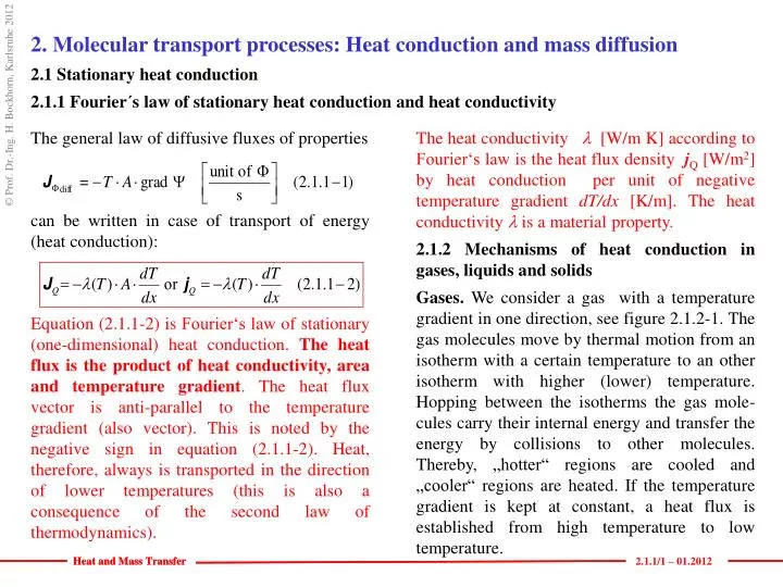
2. Moleculartransportprocesses: Heatconductionandmassdiffusion 2.1 Stationaryheatconduction 2.1.1 Fourier´slawofstationaryheatconductionandheatconductivity The general law of diffusive fluxes of properties can be written in case of transport of energy (heat conduction): Equation (2.1.1-2) is Fourier‘s law of stationary (one-dimensional) heat conduction. The heat flux is the product of heat conductivity, area and temperature gradient. The heat flux vector is anti-parallel to the temperature gradient (also vector). This is noted by the negative sign in equation (2.1.1-2). Heat, therefore, always is transported in the direction of lower temperatures (this is also a consequence of the second law of thermodynamics). The heat conductivity l [W/m K] according to Fourier‘s law is the heat flux density jQ [W/m2] by heat conduction per unit of negative temperature gradient dT/dx [K/m]. The heat conductivity l is a material property. 2.1.2 Mechanisms of heat conduction in gases, liquids and solids Gases. We consider a gas with a temperature gradient in one direction, see figure 2.1.2-1. The gas molecules move by thermal motion from an isotherm with a certain temperature to an other isotherm with higher (lower) temperature. Hopping between the isotherms the gas mole-cules carry their internal energy and transfer the energy by collisions to other molecules. Thereby, „hotter“ regions are cooled and „cooler“ regions are heated. If the temperature gradient is kept at constant, a heat flux is established from high temperature to low temperature. 2.1.1/1 – 01.2012

x T Gaseous molecules accumulate their internal energy in form of kinetic energy (translation), rotational energy and oscillation energy (the latter forms only in multi-atom molecules, e.g. H2O, N2, CO2….). Rotational energy and oscillation energy are quantized. Heat conductivity of gases. According to the simple model of heat conduction, the heat conductivity l of ideal gases can be desribed with the kinetic theory of gases: In equation (2.1.2-1) L is the mean free pass of the molecules and the mean molecular velocity of the molecules. Then: Fig. 2.1.2-1: Simple model for explication of heat conduction in gases. According to equation (2.1.2-3) the heat conductivity increases with increasing temperature (for atoms T0,5) and with increasing molar mass. According to the kinetic theory of gases, there is no pressure dependence of the heat conductivity for ideal gases. Table 2.1.2-1 contains the heat conductivities of some gases. From the table a slight pressure dependence of the heat conductivity can be seen (in contrast to the simple kinetic gas theory). 2.1.2/1 – 01.2012

Table 2.1.2-1: Heat conductivity of some gases. Table 2.1.2-2: Heat conductivity of some liquids. 2.1.2/2 – 01.2012

Heat conductivity of liquids. The mechanism of heat conduction in liquids is similar to that of heat conduction in gases, however, the interactions of molecules play an important role (hydrogen bridge bonds, van der Waals interactions, other long range and short range interactions). Table 2.1.2-2 gives an overview about the heat conductivities of some liquids. The heat conductivity of most liquids is one order of magnitude higher than the heat conductivity of gases. Water and other inorganic fluids (ammonia) exhibit a much higher heat conductivity than organic fluids; molten salts show even higher heat conductivities. The heat conductivity of liquids increases generally with increasing temperature. Simple model for heat conduction in solids. In solids molecules (lattice building blocks) cannot move freely. Tey are fixed at their lattice places, see figure 2.1.2-2. Solids store thermal energy in form of oscillations of the atoms about their rest positions in the lattice. In solids the transport of energy occurs via the oscillations of neigh-boring molecules. All molecules in the solid form a system of coupled oscillators (same mechanism as the transport of sound in solids). Fig. 2.1.2-2: Simple model for explication of heat conduction in solids. 2.1.2/3 – 01.2012

The energy quanta released or accepted from this system of coupled oscillators are called phonons. Therefore, heat conduction in solids is accomplished by transport of phonons. In addition, in metals and electrical conductors the transport of phonons is superimposed by the transport of electrons in the conductivity bond. Therefore, heat conductivity in solids is caused by the transport of phonons and the thermal movement of conductivity electrons. The latter effect increases the heat conductivity. The heat conductivity of metals is two to three orders of magnitudes higher than that of gases. Metals show a much higher thermal conductivity compared with other solids. Heat conductivities of metals correspond to electrical conductivities (Fe < Al < Cu< Ag); Wiedemann-Franz-Lorenz law. contribution of conductivity electrons to heat conduction. (k: electrical conductivity in (Wm)-1). Figure 2.1.2-3 exhibits the temperature dependency of the heat conductivity of some solids.Table 2.1.2-3 gives some values for the heat conductivity of solids. For metals and other electrical conductors the heat conductivity is a complicated function of temperature. Difference between electrical conductors and semi-conductors and insolaters in the temperature dependency of the heat conduction. Often the heat conductivity is non isotropic (graphite, wood). Detailed information about heat conductivities of different materials, methods of estimation and methods of calculation can be found in VDI-Wärmeatlas. 2.1.2/4 – 01.2012

Fig. 2.1.2-3: Temperature dependency of the heat conductivity of some solids. Table 2.1.2-3: Heat conductivities of some solids. 2.1.2/5 – 01.2012

s1 T A JQ l1 x 2.1.3 Stationaryheatconduction in planarand non-planar geometries, heattransfercoefficient Stationaryheatconductionthroughplanar geometries.Weconsider a planarplatewithhomogeneous material properties, seefigure 2.1.3-1. Boundaryconditionsattheleftandrightsurfacearekeptatconstanttemperatures. Heatconductivityisl1 . UsingFourier‘slawweobtain: Assumingl1beingconstantseparationof variables leadsto: Integration withinboundaries 0 andxresults in: Forthisproblemweobtain a linear decreaseof temperature withintheplate. l1 increasing with tempe-rature T1 l1 decreasing with tempe-rature T2 Fig. 2.1.3-1:Stationary heat conduction in planar geometries. Setting x = s1 and T(s1) = T2 and resolving for JQ gives: For l1 varying with temperature, no linear temperature profile! Heat flux 0, if l0, Heat flux  0, if s  ∞, Heat flux 0, if DT 0. 2.1.3/1 – 01.2012

T r JQ Ri Ra Ti Stationary heat conduction in spherical shells. We consider a spherical shell which is treated as one-dimensional problem (coordinate radius r). The temperatures at the inner and outer surface are constant in time and surface, see figure 2.1.3-2. The material has the heat conductivity l1. According to Fourier‘s law we write: In this case the area increases with radius. Therefore, according to Fourier‘s law we expect a steeper decrease of the temperature. Again the total heat flux is constant. Separation of variables in equation (2.1.3-4) gives: Integration within the boundaries Riand r gives: The temperature in the sperical shell varies hyperbolicly with the radius r(at constant heat conductivity, compare planar problem: linear). Ta l1 Fig. 2.1.3-2:Stationary heat conduction in non-planar geometries (sperical shells). Setting in equation (2.1.3-6) r =Ra and T(Ra) = Ta and resolving for the heat fluxJQwe obtain: With this we obtain the same form for the heat conduction equation as in the planar geometry. 2.1.3/2 – 01.2012

T R --> ∞ T = Ta r JQ Ri At otherwise constant conditions (DT, s, l1) the heat flux in spherical geometries is smaller compared to planar geometries. For Ra >> Ri in equation (2.1.3-6) 1/Ra may be neglected against1/Ri. Using this we obtain: Ti Even at high wall thicknesses (strong isolation) a minimum residual heat flux remains in spherical shell geometries according to equation (2.1.3-8). l1 Heat flux --> 0, if l -->0, Heat flux --> 0, ifDT --> 0, Heat flux--> minimum heat flux, if s --> ∞. Fig. 2.1.3-3: Introduction of the heat transfer coefficient. Heat transfer coefficient. We consider the problem analogous to heat conduction in a spherical shell, figure 2.1.3-2. The cavity is now filled with material and the shell thickness is extended to infinity. The surface temperature of the sphere (filled cavity) is constant and the temperature far away from the surface is also kept at constant, see figure 2.1.3-3. The shell material (which is now the surrounding of the sphere) has the heat conductivity l1. This scenario describes the heat transfer from a sphere into surroundings at rest. 2.1.3/3 – 01.2012

T R --> ∞ T = Ta r JQ Ri For this problem a heat transfer coefficient a is defined according to: or: With and and equa-tion (2.1.3-8) we obtain Ti l1 Generally, the heat transfer coefficient is „non-dimensionalized“ with a characteristic length L and the heat conductivity l: This number is called Nusselt number. For the problem of heat transfer from a sphere into a surrounding at rest we obtain: Fig. 2.1.3-4: Introduction of the heat transfer coefficient. With the help of the heat transfer coefficient a given in equation (2.1.3-9) any heat transfer problem can be now written as: 2.1.3/4 – 01.2012

s1 s2 T A JQ JQ JQ l1 l2 x s3 2.1.4 Stationaryheatconduction in layeredmaterials, over all heattransfercoefficient Stationaryheatconduction in layeredmaterials.Weconsider a planarbodyconsistingoflayersof different materials. The over-all thicknessissmallcomparedwiththe lateral dimensions, so thattheproblemcanbetreatedas a one-dimensional heatconductionproblem. Attheleftandright wall constanttemperaturesareapplied, seeefigure 2.1.4-1. The different layershavetheheatconductivitiesl1 ,l2andl2. ApplyingFourier‘slawweobtain: and and Resolvingforthetemperaturedifferencesandaddingresults in: T1 T1/2 T2/3 T3 l3 Fig. 2.1.4-1:Stationary heat conduction in planar layered materials. or 2.1.4/1 – 01/2012

s1 s2 T A JQ JQ JQ l1 l2 x s3 From equations (2.1.4-1) to (2.1.4-3) we find that the temperature differences in the single layers are inversely proportional to the heat conductivities per unit lenght (insolation problem). Over-all heat transfer coefficient. For the stationary heat conduction problem through a layered material we define an over-all heat transfer coefficient k similar to the heat transfer coefficient in section 2.1.3: T1 T1/2 T2/3 T3 l3 Fig. 2.1.4-1:Stationary heat conduction in planar layered materials. The heat transfer coefficients according to equations (2.1.4-8) to (2.1.4-10) are heat conductivities normalized to the thickness of the layers (specific conductivities). Then the reciprocal of the heat transfer coefficients are specific resistances (analogy to conduction of electricity). 2.1.4/2 – 01.2012

Using equations (2.1.4-8) to (2.1.4-10) in equation (2.1.4-5) yields: or With For heat conduction through „heat conduction resistances“ in series the single resistances add to the total resistance! (reciprocal specific conductivities, see figure 3.1.4-2). For heat conduction through „heat conduction resistances“ in parallel the single specific conductivities add to the total conductivity! (reciprocal specific restistances, see figure 3.1.4-3). JQ Fig. 2.1.4-2: „Heat conduction resistances“ in series. JQ 1 JQ 2 JQ 3 Fig. 2.1.4-3: „Heat conduction resistances“ in parallel. 2.1.4/3 – 01.2012

T L JQ JQx JQx+Dx JQüb x 2.1.5 Examplesofstationaryheatconduction in engineering Heatconduction in slabswithheattransferintotheambient.Weconsider a cylindricalslabwiththelengthL, mountedperpendicularto a surface. The surfaceiskeptat temperature T0andtheambient temperature isTa. The material hastheheatconductivityl, see fig. 2.1.5-1 („thermal orcoldbridge“). Problem: Temperature distribution in the slab, heat loss by the slab (thermal bridge, cold bridge). For the calculation of the temperature profile in the slab we consider a heat balance for a differential volume of the slab. Within the slab we have heat conduction, at the surface we have heat transfer to the ambient. (Simplification: temperature constant over the radius (1-d problem). Heat balance: Heat flux in = heat flux out (2.1.5-1) Heat flux into the balance volume: Heat flux out of the balance volume: T0 x x+Dx l Ta Fig. 2.1.5-1: Stationary heat conduction in a cylindrical slab. Heat transfer to the ambient (U: circumference): Heat balance for stationary conditions: 2.1.5/1 – 01.2012

T T0 L Ta x x+Dx JQ l JQx+Dx JQx JQüb x Heat flux at x+Dx is obtained by a Taylor series expansion of the heat flux at x (linearisation): For the heat balance we obtain: Transformation with q = (T-Ta)/(T0-Ta) and h = x/L gives: In equation (2.1.5-8) m2 = 4L(aaussen/l)(L/D). The ratio (aaussenR/l) can be understood as ratio of the heat transfer resistance slab/wall to wall/ambient. This ratio is called Biot number, Bi. Then m2 = 8 (L/D)2 Bi (Bi must be small for 1-d problem). Solution of the ordinary differential equation of second order (2.1.5-8): Fig. 2.1.5-1: Stationary heat conduction in a cylindrical slab. Differentiating equation (2.1.5-9) twice by h gives: Equation (2.1.5-9) is a solution of (2.1.5-8) only if 2.1.5/2 – 01.2012

General solutions: linear combination of particular solutions: Integrations constants A and B form boundary conditions. Boundary condition 1: For h = 0T =T0, therefore q = 1. This gives: Boundary condition 2: Finite long slab, heat transfer to the ambient at the front end side negligible. Then dq/dh = 0, forh = 1. This gives: Considering equation (2.1.5-13) we have: Fig. 2.1.5-2: Solution according to equation (2.1.5-16) for stationary heat conduction in a cylindrical slab (m = 5). The solution then is: 2.1.5/3 – 01.2012

Heat loss via the „cold bridge“ to the ambient as heat transfer problem: The total heat flux from the slab is supplied by heat conduction from the wall to the slab (see fig. 2.1.5-1). Therefore The heat supplied by heat conduction into the slab is transferred to the ambient. Therefore, JQ = JQüb. Solution for the temperature distribution for the stationary problem at x  0: With this we obtain from equation (2.1.5-17): On the other hand, the heat transfer problem can be formulated based on the fundamental heat transfer equation (2.1.3-14): Comparing equations (2.1.5-19) and (2.1.5-20) we obtain: We learn from this example that heat transfer from the slab to the ambient and heat conduction into the slab are coupled processes that affect each other! 2.1.5/4 – 01.2012

T JQ x Exact temperature measurement. We mount a temperature sensor (thermo couple) into the slab to measure the temperature Ta. How close is the temperature at the front end to the ambient temperature Ta? In this case Ta > T0. T0 Ta For the front end of the slab (h = 1) we obtain: For the measuring error to be smaller than 0,5% we have: Transformation gives: Finally: Example: a = 100 W/m2 K, l = 60 W/m K, U/A = 1/s, s = 1 mm. TL l Fig. 2.1.5-3: For the demonstration of the thermometry problem. Then For the prevailing conditions the slab has to have a length of minimum 15 cm! 2.1.5/5 – 01.2012

Summaryofsection 2.1 • The different mechanismsofheatconductionhavebeenqualitativelydiscussed. • The basicsofheatconduction in fluidsandsolidshavebeenelaborated. • The material property „heatconductivity“ hasbeendiscussed. • The heattransfercoefficienthasbeenintroduced. • The over all heattransfercoefficienthasbeenintroduced. • Stationaryheatconductionfor different geometries andsomeproblemsfromprocessengineeringhasbeenelucidated. 2.1.5/6 – 01.2012

T JQ JQ(x+Dx) JQ(x) JQüb JQacc x 2.2 Non stationaryheatconduction 2.2.1 Fourier‘slawof non stationaryheatconductionand thermal conductivity Uptonowonlystationaryheatconductionproblemshavebeendiscussed. Forthisproblemstemperaturesandheatfluxesare invariant against time. In processtechnologymostproblemsare non stationary, so that non stationaryheatconductionhastobediscussed in thefollowing. Basics of non stationary heat conduction; Fourier‘s law of non stationary heat conduction. Again we consider a cylindrical slab with homogeneous material properties (l, cp, r) which is mounted at a wall. (Simplification: temperature constant over the radius (1-d problem). The wall temperature is initially Ta and is increased at t = 0 to T0. The temperature distribution and heat fluxes are now dependent on distance and time! For determinationof the temperature distribution in the slab we consider the heat balance for a differential volume of the slab. Within the slab we have heat conduction and accumulation, at the surface we have heat transfer to the ambient. Heat balance: accumulation of heat = heat flux in – heat flux out (2.2.1-1) T0 x x+Dx l Ta Fig. 2.2.1-1:For derivation of Fourier‘s law for non stationary heat conduction. 2.2.1/1 – 01.2012

T JQ JQ(x+Dx) JQ(x) JQüb JQacc x Heat flux into the balance volume by heat conduction: Heat flux out of the balance volume by heat conduction: Heat transfer to the ambient (U: circumference): Accumulation of heat: T0 x x+Dx l Ta Fig. 2.2.1-1:For derivation of Fourier‘s law for non stationary heat conduction. Heat balance for non stationary conditions: 2.2.1/2 – 01.2012

Heat balance results in: Temperature gradient is expanded into a Taylor series (linearization of the temperature gradient): Using this in the heat balance gives: Transformation results in: For aaussen --> 0, no heat transfer to the ambient, we obtain Fourier‘s law for non stationary heat conduction: The property a = l/r cp [m2/s] is called thermal conductivity (temperaure conductivity). It is a material property. Some values are given in table 2.2.1-1. Table 2.2.1-1:Thermal conductivities of some materials. 2.2.1/3– 01.2012

T0 T l JQ Ta x 2.2.2 Examplesof non stationaryheatconduction in engineering Solutions ofFourier‘s differential equationfor non stationaryheatconduction. Geometry: cylindricalslabwith L/D >> 1, thenTL = Ta, forthe time beingnoheattransfertotheambient. Initial and boundary conditions: Normalization of temperature q = (T-Ta)/(T0-Ta) gives: Initial and boundary conditions : Approach for solution: partial differential equation is transferred into an ordinary differential equation by use of a new variable which connects time and distance. For transformation the Fourier number is introduced: Fig. 2.2.2-1: Non stationary heat conduction in a cylindrical slab. The Fourier number has the meaning of a normalized time: a/x2: „Intrusion time“ for temperature. New variable: 2.2.2/1– 01.2012

T0 T l JQ Ta x Transformation rules: Considering the transformation rules we obtain from the heat conduction equation: And after transformation: Finally we obtain by further transformation a system of coupled ordinary differential equations of first order: Fig. 2.2.2-1: Non stationary heat conduction in a cylindrical slab. Integration of the first equation after separation of variables considering the boundary condition Y = Y0 for f = 0: Integration of the second equation within the boundaries f = 0 and f and 1 und q , respectively, yields: 2.2.2/2– 01.2012

The integral in equation (2.2.2-16) is given by p1/2/2.erf(f), where erf(f) is the error function. The remaining task is the determination of the wall gradient in equation (2.2.2-16) (dq/df)0. The error function erf(f) converges assymptoticly at large f versus 1. Therefore p1/2/2.erf(f) converges against 0,8862, compare figure 2.2.2-2. From equation (2.2.2-16) we then obtain for large f (q = (T-Ta)/(T0-Ta)=0): Or: The general solution of the non stationary heat conduction equation for the cylindrical slab with the above initial and boundary conditions then is: Fig. 2.2.2-3: Temperature distribution according to equation (2.2.2-19). Fig. 2.2.2-2: Error function erf(f). 2.2.2/3– 01.2012

T0 JQÜbertragung T l JQ Ta x Solutions of Fourier‘s differential equation for non stationary heat conduction. Geometry: cylindrical slab with L/D >> 1, then TL = Ta, now with heat transfer to the ambient! Initial and boundary conditions identical to the case without heat transfer to the ambient. Normalization of temperature as bevor with q = (T-Ta)/(T0-Ta) gives: with n=(aaussen/cpr)(4/D). Initial and boundary conditions: If the solution for n = 0 is then the solution for is (Dankwerts, Crank): Fig. 2.2.2-4: Non stationary heat conduc-tion in a cylindrical slab with heat trans-fer to the ambient. Solution: 2.2.2/4– 01.2012

T0 JQÜbertragung T l JQ Ta x Heat loss via the „cold bridge“ to the ambient for non stationary conditions as heat transfer problem:The total heat flux from the slab is supplied by heat conduction from the wall to the slab (see fig. 2.2.2-5). From equation (2.2.2-18) we obtain (for the case without heat transfer to the ambient): On the other hand, the heat transfer problem can be formulated with the help of the fundamental heat transfer equation: Comparing equation (2.2.2-26) and (2.2.2-27) we obtain In this case the heat transfer coefficient for the heat loss via the „cold bridge“ is time dependent! Fig. 2.2.2-5: Non stationary heat conduction in a cylindrical slab (a = 2.10-5 m2 s-1, n = 10-3 s-1). 2.2.2/5– 01.2012

For t  large error function  1 and exp(-nt)  0, so that Averaging the heat transfer coefficient for the non stationary problem over time gives: The averaged heat transfer coefficient is exactly double of the instantaneous heat transfer coefficient at time t. For the case including heat transfer to the ambient (coupled inner and outer heat transfer) we obtain: The heat transfer coefficient the is given by: For t  0 error function  0 and exp(-nt)  1, so that Fig. 2.2.2-6: Non stationary heat conduction in a cylindrical slab (a = 2.10-5 m2 s-1, n = 10-3 s-1); heat transfer coefficients. 2.2.2/6– 01.2012

Summary section 2.2 • Fundamentals of non-stationary heat conduction have been deduced. • A method for the solution of the partial differential equation for non-stationary heat conduction has been discussed. • Definition of the heat transfer coefficient has been extended to non-stationary heat conduction problems. 2.2.2/7– 01.2012

Diffusionflux of A Diffusionflux of B x 2.3 Stationary diffusion 2.3.1 Fick´s law of stationary diffusion and diffusion coefficient The general law of diffusive fluxes of properties can be written in case of transport of chemical species (diffusion): Equation (2.3.1-2) is Fick‘s law of stationary diffuison. The mole flux of species k is the product of diffusion coefficient, area and concentration gradient. The mole flux vector is anti-parallel to the concentration gradient, negative sign in equation (2.1.1-2). The species k, therefore, always is transported in the direction of lower concentrations. The diffusion coefficient D [m2/s] according to Ficks‘s law is the mole flux density jnk [mole/m2.s] by diffusion per unit of negative concentration gradient dck/dx [mole/m4]. The diffusion coefficient D is a material property. 2.3.2 Mechanisms of diffusion Simple model for diffusion in a fluid (gas, liquid). Fluid particles (molecules in a gas) move driven by thermal molecular motion with a temperature dependent velocity. During this motion the molecules strike each other. Every strike leads to a change of the direction of the motion, so that the molecules in the average at constant pressure and constant temperature move homogeneously in all directions. cA > cB cA < cB Fig. 2.3.2-1:Simple model for the explanation of diffusion. 2.3.1/1 – 01.2012

_ If in a closed system a concentration gradient for the single molecules exists, compare figure 2.3.2-1, on the time average more molecules from the region of higher concentration will move into the region of lower concentration. By this a diffusion flux is established into the direction of lower concentrations. According to that simple model, the diffusion coefficient should be dependent on the mean molcular velocity and the mean free path of the molecules and from that on temperature and pressure. Diffusion coefficients of gases. According to the above simple model for the diffusion of gases the diffusion coefficient of ideal gases can be calculated with the help of the kinetic gas theory: In equation (2.3.2-1) L is the mean free path of the molecules and v the mean molecular velocity (compare heat conductivity). According to equation (2.3.2-4), kinetic gas theory, the diffusion coefficients increase with decreasing molar mass of the molecules. Increasing temperatures lead to a strong increase of the diffusion coefficients (T1,5). According to the kinetic gas theory we have a pressure dependence according to p-1. Diffusion coefficients of liquids. The diffusion coefficients of most liquids are about five orders of magnitude lower than those of gases. The mechanism of diffusion in liquids is similar to the mechnism of diffusion in gases. However, the interactions of the molecules in the fluid (van der Waals interactions, hydrogen bridge bonds, long distance interactions) play an important role. Thereby, the diffusion coefficients of most species in liquids are dependent on concentration, compare table 2.3.2-2. 2.3.2/2 – 01.2012

Table 2.3.2-1:Binary diffusion coefficients for some gas mixtures. Diffusion coefficients of solids. The mechanism of diffusion in solids is much more complicated (diffusion of empty places in the lattice, etc.). Table 2.3.2-2: Diffusion coefficients of some fluid mixtures. 2.3.2/3 – 01.2012

x+Dx x cAS cA JnA(x+Dx) JnA(x) DA x 2.4 Non-stationary diffusion 2.4.1 Fick‘s law for non-stationary diffusion Analogously to non stationary heat conduction we can derive the differential equation for non stationary diffusion with the help of a mass balance for the scenario given in figure 2.4.1-1. We focus again on a planar diffusion problem (e.g. solution of a solid in water), which can be treated 1-dimensionally. In the fluid initially a constant concentration cA0prevails, compare figure 2.4.1-1. At time t = 0 the concentration is sudddenly increased to cAS (immersion of the solid into water). An equation of the evolution of the concentration cA with time is obtained from a mass balance for species A in a differential balance volume: Accumulation of moles of A = inflow of moles of A – outflow of moles of A (2.4.1-1) In the same way as for non stationary heat conduction we obtain finally Fig. 2.4.1-1: Mass balance for derivation of Fick‘s law for non-stationary diffusion. Equation (2.4.1-2) is Fick‘s law for non-stationary diffusion and is (formal) identical to the equation for non-stationary heat conduction! The solutions of this equation then are identical to the solutions of the equation for non-stationary heat conduction (if initial and boundary conditions are identical). 2.4.1/1 – 01.2012

2.5 Similarity of heat and mass transfer As can be seen from equations (2.1.1.-2), (2.2.2-1), (2.3.1-2) and (2.4.1-2) heat transport by (stationary and non stationary) conduction and mass transport by (stationary and non stationary) diffusion are closely related with vast analogies: Also, the transport coefficients (heat conductivity, diffusion coefficients) are closely related, e.g. from kinetic theory of gases we obtain for ideal gases: This gives then: Due to this similarity, heat transfer problems and mass transfer problems can be often treated similarly! general heat transfer equation ! general mass transfer equation ! 2.5/1 – 01.2012

c L Jn Jnx Jnx+Dx JnReaktion x 2.6 Examples for stationary diffusion problems from process engineering Diffusion into a porous catalyst with simultaneous chemical reaction. In a pellet of a catalysts we have round pores of the length L, into which from the surface of the pellet a chemical component diffuses and reacts at the inner surface of the pore. The pores can be treated for simplicity as cylinders. At the outer surface the concentration is c0, compare figure 2.6-1. The diffusion coefficient of the species is DA. Question: concentration profile in the pore of the catalyst, molar flux into the catalyst. We perform a mass balance for the species A over a differential balance volume. Within the pore we have diffusion of the species A and the species A reacts at the wall of the pore into products according to a chemical reaction of first order. (Simplification: concentration only dependent on x, 1-dimensional problem.) Mass balance: Diffusion flux of A into the volume: Diffusion flux of A out of the volume: x x+Dx c0 DA c Fig. 2.6-1: Stationary diffusion into a round pore of a catalyst. Reaction of A in the volume by heterogeneous chemical reaction (U: pore circumference): 2.6/1 – 01.2012

c L x x+Dx c0 Jn DA Jnx Jnx+Dx JnReaktion c x Mass balance for stationary conditions: The molar flux at the position x+Dx is replaced by a Taylor series of the molar flux at the position x: With this we have for the mass balance: Transformation using q = c/c0 and h = x/L gives: In equation (2.6-8) m2 = (k.U.L2)/(DA.A) = L2(2k/DA.R) = f2. f is called the Thiele-Modulus. The Thiele modulus can be interpreted as ratio of reatcion rate to diffusion rate. Solution of the ordinary differential equation of second order for q: el-Ansatz: Fig. 2.6-1: Stationary diffusion into a round pore of a catalyst. Differentiating with respect to h gives: Equation (2.6-9) is therefore only a solution of equation (2.6-8) if: 2.6/2 – 01.2012

General solution: linear combination of the particular solutions: The integration constants A and B are calculated from the boundary conditions. Boundary condition 1: For h = 0 is c =c0, therefore q = 1. This gives: Boundary condition 2: The end of the pore is not permeable for material. Then dq/dh = 0, forh = 1. Then it follows: With equation (2.6-13) we obtain: The solution then is: Fig. 2.6-2: Solution of equation (2.6-8) for stationary diffusion in a pore of a catalyst. With increasing Thiele modulus, that is with increasing reaction rate compared to the diffusion rate, the concentration decreases steeper and the concentration gradient at the outer surface increases. 2.6/3 – 01.2012

Diffusion into the pores as mass transfer problem: The mass of the component A which is consumed by chemical reaction within the pore of the catalyst has to be transportet through the pore entrance by diffusion. Therefore Concentration profile for the stationary problem: This gives: On the other hand, every mass transfer problem – in this case the mass transfer from the outer surface of the catalyst into the inner of the pore – can be written as (compare equation 2.5-3): Comparing equation (2.6-19) and (2.6-20) we obtain (with coo = 0 for m>5): The mass transfer through the pore entrance of the catalyst and the chemical reaction at the inner surface are coupled ! The faster the chemical reaction (the larger the Thiele modulus) the larger is the mass transfer coeffcient ! (compare stationary heat conduction in a slab ?) 2.6/4– 01.2012

Summary sections 2.3 to 2.6 • The different mechanisms of diffusion have been discussed. • Basics of diffusion in fluids have been elaborated. • The property „diffusion coefficient“ has been discussed. • Stationary diffusion has been terated. • Non stationary diffusion has been introduced • Similarity between heat transport and mass transport has been identified. • Simple problems for diffusion from process engineering have been discussed. 2.6/5– 01.2012

2. Molecular transport processes : Heat conduction and mass diffusion