Download
1 / 53
530 likes | 662 Vues
Chapter 1 Data and Statistics. I need help!. Applications in Business and Economics. Data. Data Sources. Descriptive Statistics. Statistical Inference. Computers and Statistical Analysis. Applications in Business and Economics. Accounting.

E N D
Chapter 1 Data and Statistics I need help! • Applications in Business and Economics • Data • Data Sources • Descriptive Statistics • Statistical Inference • Computers and Statistical Analysis
Applications in Business and Economics • Accounting Public accounting firms use statistical sampling procedures when conducting audits for their clients. • Economics Economists use statistical information in making forecasts about the future of the economy or some aspect of it.
Applications in Business and Economics • Marketing Electronic point-of-sale scanners at retail checkout counters are used to collect data for a variety of marketing research applications. • Production A variety of statistical quality control charts are used to monitor the output of a production process.
Applications in Business and Economics • Finance Financial advisors use price-earnings ratios and dividend yields to guide their investment recommendations.
Data and Data Sets • Data are the facts and figures collected, summarized, analyzed, and interpreted. • The data collected in a particular study are referred • to as the data set.
Elements, Variables, and Observations • The elements are the entities on which data are collected. • A variable is a characteristic of interest for the elements. • The set of measurements collected for a particular element is called an observation. • The total number of data values in a complete data set is the number of elements multiplied by the number of variables.
Data, Data Sets, Elements, Variables, and Observations Variables Observation Element Names Stock Annual Earn/ Exchange Sales($M) Share($) Company NQ 73.10 0.86 N 74.00 1.67 N 365.70 0.86 NQ 111.40 0.33 N 17.60 0.13 Dataram EnergySouth Keystone LandCare Psychemedics Data Set
Scales of Measurement Scales of measurement include: Nominal Interval Ordinal Ratio The scale determines the amount of information contained in the data. The scale indicates the data summarization and statistical analyses that are most appropriate.
Scales of Measurement • Nominal Data are labels or names used to identify an attribute of the element. A nonnumeric label or numeric code may be used.
Scales of Measurement • Nominal Example: Students of a university are classified by the school in which they are enrolled using a nonnumeric label such as Business, Humanities, Education, and so on. Alternatively, a numeric code could be used for the school variable (e.g. 1 denotes Business, 2 denotes Humanities, 3 denotes Education, and so on).
Scales of Measurement • Ordinal The data have the properties of nominal data and the order or rank of the data is meaningful. A nonnumeric label or numeric code may be used.
Scales of Measurement • Ordinal Example: Students of a university are classified by their class standing using a nonnumeric label such as Freshman, Sophomore, Junior, or Senior. Alternatively, a numeric code could be used for the class standing variable (e.g. 1 denotes Freshman, 2 denotes Sophomore, and so on).
Scales of Measurement • Interval The data have the properties of ordinal data, and the interval between observations is expressed in terms of a fixed unit of measure. Interval data are always numeric.
Scales of Measurement • Interval Example: Melissa has an SAT score of 1205, while Kevin has an SAT score of 1090. Melissa scored 115 points more than Kevin.
Scales of Measurement • Ratio The data have all the properties of interval data and the ratio of two values is meaningful. Variables such as distance, height, weight, and time use the ratio scale. This scale must contain a zero value that indicates that nothing exists for the variable at the zero point.
Scales of Measurement • Ratio Example: Melissa’s college record shows 36 credit hours earned, while Kevin’s record shows 72 credit hours earned. Kevin has twice as many credit hours earned as Melissa.
Qualitative and Quantitative Data Data can be further classified as being qualitative or quantitative. The statistical analysis that is appropriate depends on whether the data for the variable are qualitative or quantitative. In general, there are more alternatives for statistical analysis when the data are quantitative.
Qualitative Data Labels or names used to identify an attribute of each element Often referred to as categorical data Use either the nominal or ordinal scale of measurement Can be either numeric or nonnumeric Appropriate statistical analyses are rather limited
Quantitative Data Quantitative data indicate how many or how much: discrete, if measuring how many continuous, if measuring how much Quantitative data are always numeric. Ordinary arithmetic operations are meaningful for quantitative data.
Scales of Measurement Data Qualitative Quantitative Numerical Numerical Non-numerical Nominal Ordinal Nominal Ordinal Interval Ratio
Cross-Sectional Data Cross-sectional data are collected at the same or approximately the same point in time. Example: data detailing the number of building permits issued in June 2007 in each of the counties of Ohio
Time Series Data Time series data are collected over several time periods. Example: data detailing the number of building permits issued in Lucas County, Ohio in each of the last 36 months
Data Sources • Existing Sources Within a firm – almost any department Business database services – Dow Jones & Co. Government agencies - U.S. Department of Labor Industry associations – Travel Industry Association of America Special-interest organizations – Graduate Management Admission Council Internet – more and more firms
Data Sources • Statistical Studies • In experimental studies the variable of interest is • first identified. Then one or more other variables • are identified and controlled so that data can be • obtained about how they influence the variable of • interest. In observational (nonexperimental) studies no attempt is made to control or influence the variables of interest. a survey is a good example
Data Acquisition Considerations Time Requirement • Searching for information can be time consuming. • Information may no longer be useful by the time it • is available. Cost of Acquisition • Organizations often charge for information even • when it is not their primary business activity. Data Errors • Using any data that happen to be available or were • acquired with little care can lead to misleading • information.
Descriptive Statistics • Descriptive statistics are the tabular, graphical, and numerical methods used to summarize and present data.
Example: Hudson Auto Repair The manager of Hudson Auto would like to have a better understanding of the cost of parts used in the engine tune-ups performed in the shop. She examines 50 customer invoices for tune-ups. The costs of parts, rounded to the nearest dollar, are listed on the next slide.
Example: Hudson Auto Repair • Sample of Parts Cost ($) for 50 Tune-ups
Tabular Summary: Frequency and Percent Frequency Parts Cost ($) Percent Frequency Parts Frequency 2 13 16 7 7 5 50 4 26 32 14 14 10 100 50-59 60-69 70-79 80-89 90-99 100-109 (2/50)100
18 16 14 12 10 8 6 4 2 Graphical Summary: Histogram Tune-up Parts Cost Frequency Parts Cost ($) 50-59 60-69 70-79 80-89 90-99 100-110
Numerical Descriptive Statistics • The most common numerical descriptive statistic • is the average (or mean). • Hudson’s average cost of parts, based on the 50 • tune-ups studied, is $79 (found by summing the • 50 cost values and then dividing by 50).
Statistical Inference Population - the set of all elements of interest in a particular study Sample - a subset of the population Statistical inference - the process of using data obtained from a sample to make estimates and test hypotheses about the characteristics of a population Census - collecting data for a population Sample survey - collecting data for a sample
Process of Statistical Inference 1. Population consists of all tune- ups. Average cost of parts is unknown. 2. A sample of 50 engine tune-ups is examined. • The sample data • provide a sample • average parts cost • of $79 per tune-up. 4. The sample average is used to estimate the population average.
Computers and Statistical Analysis • Statistical analysis typically involves working with • large amounts of data. • Computer software is typically used to conduct the • analysis. • Instructions are provided in chapter appendices for carrying out many of the statistical procedures using Minitab and Excel.
Sampling Distribution of Chapter 7, Part ASampling and Sampling Distributions • Simple Random Sampling • Point Estimation • Introduction to Sampling Distributions
Statistical Inference The purpose of statistical inference is to obtain information about a population from information contained in a sample. A population is the set of all the elements of interest. A sample is a subset of the population.
Statistical Inference The sample results provide only estimates of the values of the population characteristics. With proper sampling methods, the sample results can provide “good” estimates of the population characteristics. A parameter is a numerical characteristic of a population.
Simple Random Sampling:Finite Population • Finite populations are often defined by lists such as: • Organization membership roster • Credit card account numbers • Inventory product numbers • A simple random sample of size n from a finite population of size N is a sample selected such that each possible sample of size n has the same probability of being selected.
Simple Random Sampling:Finite Population • Replacing each sampled element before selecting • subsequent elements is called sampling with • replacement. • Sampling without replacement is the procedure • used most often. • In large sampling projects, computer-generated • random numbers are often used to automate the • sample selection process.
Simple Random Sampling:Infinite Population • Infinite populations are often defined by an ongoing process whereby the elements of the population consist of items generated as though the process would operate indefinitely. • A simple random sample from an infinite population is a sample selected such that the following conditions are satisfied. • Each element selected comes from the same • population. • Each element is selected independently.
Simple Random Sampling:Infinite Population • In the case of infinite populations, it is impossible to • obtain a list of all elements in the population. • The random number selection procedure cannot be • used for infinite populations.
We refer to as the point estimator of the population mean . is the point estimator of the population proportion p. Point Estimation In point estimation we use the data from the sample to compute a value of a sample statistic that serves as an estimate of a population parameter. s is the point estimator of the population standard deviation .
Other Sampling Methods • Stratified Random Sampling • Cluster Sampling • Systematic Sampling • Convenience Sampling • Judgment Sampling
Stratified Random Sampling The population is first divided into groups of elements called strata. Each element in the population belongs to one and only one stratum. Best results are obtained when the elements within each stratum are as much alike as possible (i.e. a homogeneous group).
Stratified Random Sampling A simple random sample is taken from each stratum. Formulas are available for combining the stratum sample results into one population parameter estimate. Advantage: If strata are homogeneous, this method is as “precise” as simple random sampling but with a smaller total sample size. Example: The basis for forming the strata might be department, location, age, industry type, and so on.
Cluster Sampling The population is first divided into separate groups of elements called clusters. Ideally, each cluster is a representative small-scale version of the population (i.e. heterogeneous group). A simple random sample of the clusters is then taken. All elements within each sampled (chosen) cluster form the sample.
Cluster Sampling Example: A primary application is area sampling, where clusters are city blocks or other well-defined areas. Advantage: The close proximity of elements can be cost effective (i.e. many sample observations can be obtained in a short time). Disadvantage: This method generally requires a larger total sample size than simple or stratified random sampling.
Systematic Sampling If a sample size of n is desired from a population containing N elements, we might sample one element for every n/N elements in the population. We randomly select one of the first n/N elements from the population list. We then select every n/Nth element that follows in the population list.
Systematic Sampling This method has the properties of a simple random sample, especially if the list of the population elements is a random ordering. Advantage: The sample usually will be easier to identify than it would be if simple random sampling were used. Example: Selecting every 100th listing in a telephone book after the first randomly selected listing
Convenience Sampling It is a nonprobability sampling technique. Items are included in the sample without known probabilities of being selected. The sample is identified primarily by convenience. Example: A professor conducting research might use student volunteers to constitute a sample.