Download
1 / 147
1.48k likes | 1.53k Vues
Artificial Intelligence Problem solving by searching CSC 361. Dr. Yousef Al-Ohali Computer Science Depart. CCIS – King Saud University Saudi Arabia yousef@ccis.edu.sa http://faculty.ksu.edu.sa/YAlohali. Problem Solving by Searching Search Methods : Uninformed (Blind) search.

E N D
Artificial IntelligenceProblem solving by searchingCSC 361 Dr. Yousef Al-Ohali Computer Science Depart. CCIS – King Saud University Saudi Arabia yousef@ccis.edu.sa http://faculty.ksu.edu.sa/YAlohali
Problem Solving by SearchingSearch Methods : Uninformed (Blind) search
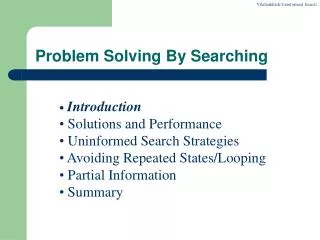
Search Methods • Once we have defined the problem space (state representation, the initial state, the goal state and operators) is all done? • Let’s consider the River Problem: A farmer wishes to carry a wolf, a duck and corn across a river, from the south to the north shore. The farmer is the proud owner of a small rowing boat called Bounty which he feels is easily up to the job. Unfortunately the boat is only large enough to carry at most the farmer and one other item. Worse again, if left unattended the wolf will eat the duck and the duck will eat the corn. How can the farmer safely transport the wolf, the duck and the corn to the opposite shore? River boat Farmer, Wolf, Duck and Corn
FWCD/- Search Methods • The River Problem: F=Farmer W=Wolf D=Duck C=Corn /=River How can the farmer safely transport the wolf, the duck and the corn to the opposite shore? -/FWCD
Search Methods • Problem formulation: • State representation: location of farmer and items in both sides of river [items in South shore / items in North shore] : (FWDC/-, FD/WC, C/FWD …) • Initial State: farmer, wolf, duck and corn in the south shore FWDC/- • Goal State: farmer, duck and corn in the north shore -/FWDC • Operators: the farmer takes in the boat at most one item from one side to the other side (F-Takes-W, F-Takes-D, F-Takes-C, F-Takes-Self [himself only]) • Path cost: the number of crossings
Search Methods • State space: A problem is solved by moving from the initial state to the goal state by applying valid operators in sequence. Thus the state space is the set of states reachable from a particular initial state. Initial state Deadends Illegal states intermediate state repeatedstate Goal state
Search Methods • Searching for a solution: We start with the initial state and keep using the operators to expand the parent nodes till we find a goal state. • …but the search space might be large… • …really large… • So we need some systematic way to search.
Search Methods • Problem solution: A problem solution is simply the set of operators (actions) needed to reach the goal state from the initial state: F-Takes-D, F-Takes-Self, F-Takes-W, F-Takes-D, F-Takes-C, F-Takes-Self, F-Takes-D.
F D D F W D F-Takes-D F-Takes-S F-Takes-W W C F W C C F W D C WC/FD FWC/D C/FWD Initial State F-Takes-D F W C W C W F W G C F-Takes-S F-Takes-C F-Takes-D F D D F D C FD/WC D/FWC FDC/W Goal State Search Methods • Problem solution: (path Cost = 7) While there are other possibilities here is one 7 step solution to the river problem
Problem Solving by searching Basic Search Algorithms
Basic Search Algorithms • uninformed( Blind) search: breadth-first, depth-first, depth limited, iterative deepening, and bidirectional search • informed (Heuristic) search: search is guided by an evaluation function: Greedy best-first, A*, IDA*, and beam search • optimization in which the search is to find an optimal value of an objective function: hill climbing, simulated annealing, genetic algorithms, Ant Colony Optimization • Game playing, an adversarial search: minimax algorithm, alpha-beta pruning
What Criteria are used to Compare different search techniques ? As we are going to consider different techniques to search the problem space, we need to consider what criteria we will use to compare them. • Completeness: Is the technique guaranteed to find an answer (if there is one). • Optimality/Admissibility: does it always find a least-cost solution? - an admissible algorithm will find a solution with minimum cost • Time Complexity: How long does it take to find a solution. • Space Complexity: How much memory does it take to find a solution.
Time and Space Complexity ? Time and space complexity are measured in terms of: • The average number of new nodes we create when expanding a new node is the (effective) branching factor b. • The (maximum) branching factor b is defined as the maximum nodes created when a new node is expanded. • The length of a path to a goal is the depth d. • The maximum length of any path in the state space m.
2 1 3 4 7 6 5 8 Branching factors for some problems • The eight puzzle has a (effective) branching factor of 2.13, so a search tree at depth 20 has about 3.7 million nodes: O(bd) • Rubik’s cube has a (effective) branching factor of 13.34. There are 901,083,404,981,813,616 different states. The average depth of a solution is about 18. • Chess has a branching factor of about 35, there are about 10120 states (there are about 1079 electrons in the universe).
A Toy Example: A Romanian Holiday • State space: Cities in Romania • Initial state: Town of Arad • Goal: Airport in Bucharest • Operators: Drive between cities • Solution: Sequence of cities • Path cost: number of cities, distance, time, fuel
Generic Search Algorithms • Basic Idea: Off-line exploration of state space by generating successors of already-explored states (also known as expanding states). Function GENERAL-SEARCH (problem, strategy) returns a solution or failure Initialize the search tree using the initial state of problem loop do if there are no candidates for expansion, then return failure Choose a leaf node for expansion according to strategy if node contains goal state then return solution else expand node and add resulting nodes to search tree. end
Arad Zerind Sibiu Timisoara Oradea Fagaras Arad Rimnicu Vilcea Sibiu Bucharest Representing Search
Implementation of Generic Search Algorithm function general-search(problem, QUEUEING-FUNCTION) nodes = MAKE-QUEUE(MAKE-NODE(problem.INITIAL-STATE)) loop do if EMPTY(nodes) then return "failure" node = REMOVE-FRONT(nodes) if problem.GOAL-TEST(node.STATE) succeeds then return solution(node) nodes = QUEUEING-FUNCTION(nodes, EXPAND(node, problem.OPERATORS)) end A nice fact about this search algorithm is that we can use a single algorithm to do many kinds of search. The only difference is in how the nodes are placed in the queue.The choice of queuing function is the main feature.
Key Issues of State-Space search algorithm • Search process constructs a “search tree” • root is the start node • leaf nodes are: • unexpanded nodes (in the nodes list) • “dead ends” (nodes that aren’t goals and have no successors because no operators were applicable) • Loops in a graph may cause a “search tree” to be infinite even if the state space is small • changing definition of how nodes are added to list leads to a different search strategy • Solution desired may be: • just the goal state • a path from start to goal state (e.g., 8-puzzle)
Uninformed search strategies (Blind search) Uninformed (blind) strategies use only the information available in the problem definition. These strategies order nodes without using any domain specific information Contrary to Informed search techniques which might have additional information (e.g. a compass). • Breadth-first search • Uniform-cost search • Depth-first search • Depth-limited search • Iterative deepening search • Bidirectional search
Basic Search AlgorithmsUninformed Search Breadth First Search (BFS)
Breadth First Search (BFS) Main idea: Expand all nodes at depth (i) before expanding nodes at depth (i + 1) Level-order Traversal. Implementation: Use of a First-In-First-Out queue (FIFO). Nodes visited first are expanded first. Enqueue nodes in FIFO (first-in, first-out) order. • Complete? Yes. • Optimal? Yes, if path cost is nondecreasing function of depth • Time Complexity: O(bd) • Space Complexity: O(bd), note that every node in the fringe is kept in the queue.
Arad Zerind Sibiu Timisoara Oradea Fagaras Arad Rimnicu Vilcea Arad Arad Oradea Lugoj Breadth First Search • QUEUING-FN:- successors added to end of queue Shallow nodes are expanded before deeper nodes.
Basic Search AlgorithmsUninformed Search Uniform Cost Search (UCS)
Uniform Cost Search (UCS) 5 2 [2] [5] 1 4 1 7 [6] [3] [9] [9] Goal state 4 5 [x] = g(n) path cost of node n [7] [8]
5 2 [2] [5] Uniform Cost Search (UCS)
Uniform Cost Search (UCS) 5 2 [2] [5] 1 7 [3] [9]
Uniform Cost Search (UCS) 5 2 [2] [5] 1 7 [3] [9] 4 5 [7] [8]
5 2 [2] [5] 1 4 1 7 [6] [3] [9] [9] 4 5 [7] [8] Uniform Cost Search (UCS)
5 2 [2] [5] Goal state path cost g(n)=[6] 1 4 1 7 [3] [9] [9] 4 5 [7] [8] Uniform Cost Search (UCS)
5 2 [2] [5] 1 4 1 7 [6] [3] [9] [9] 4 5 [7] [8] Uniform Cost Search (UCS)
Uniform Cost Search (UCS) • In case of equal step costs, Breadth First search finds the optimal solution. • For any step-cost function, Uniform Cost search expands the node n with the lowest path cost. • UCS takes into account the total cost: g(n). • UCS is guided by path costs rather than depths. Nodes are ordered according to their path cost.
Uniform Cost Search (UCS) • Main idea: Expand the cheapest node. Where the cost is the path cost g(n). • Implementation: Enqueue nodes in order of cost g(n). QUEUING-FN:- insert in order of increasing path cost. Enqueue new node at the appropriate position in the queue so that we dequeue the cheapest node. • Complete? Yes. • Optimal? Yes, if path cost is nondecreasing function of depth • Time Complexity: O(bd) • Space Complexity: O(bd), note that every node in the fringe keep in the queue.
Basic Search AlgorithmsUninformed Search Depth First Search (DFS)
Depth First Search (DFS) Main idea: Expand node at the deepest level (breaking ties left to right). Implementation: use of a Last-In-First-Out queue or stack(LIFO).Enqueue nodes in LIFO (last-in, first-out) order. • Complete? No (Yes on finite trees, with no loops). • Optimal? No • Time Complexity: O(bm), where m is the maximum depth. • Space Complexity: O(bm), where m is the maximum depth.
Arad Zerind Zerind Sibiu Sibiu Timisoara Timisoara Arad Oradea Depth-First Search (DFS) • QUEUING-FN:- insert successors at front of queue
Basic Search AlgorithmsUninformed Search Depth-Limited Search (DLS)
Depth-Limited Search (DLS) Depth Bound = 3
Depth-Limited Search (DLS) It is simply DFS with a depth bound. • Searching is not permitted beyond the depth bound. • Works well if we know what the depth of the solution is. • Termination is guaranteed. • If the solution is beneath the depth bound, the search cannot find the goal (hence this search algorithm is incomplete). • Otherwise use Iterative deepening search (IDS).
Depth-Limited Search (DLS) • Main idea: Expand node at the deepest level, but limit depth to L. • Implementation: • Enqueue nodes in LIFO (last-in, first-out) order. But limit depth to L • Complete? Yes if there is a goal state at a depth less than L • Optimal? No • Time Complexity: O(bL), where L is the cutoff. • Space Complexity: O(bL), where L is the cutoff.
Basic Search AlgorithmsUninformed Search Iterative Deepening Search (IDS)
Iterative Deepening Search (IDS) function ITERATIVE-DEEPENING-SEARCH(): for depth = 0 to infinity do if DEPTH-LIMITED-SEARCH(depth) succeeds then return its result end return failure
Iterative Deepening Search (IDS) • Key idea: Iterative deepening search (IDS) applies DLS repeatedly with increasing depth. It terminates when a solution is found or no solutions exists. • IDS combines the benefits of BFS and DFS: Like DFS the memory requirements are very modest (O(bd)). Like BFS, it is complete when the branching factor is finite. • The total number of generated nodes is : N(IDS)=(d)b + (d-1) b2 + …+(1)bd • In general, iterative deepening is the preferred uninformed search method when there is a large search space and the depth of the solution is not known.
Iterative Deepening Search (IDS) L = 0 L = 1 L = 2 L = 3