Download
1 / 28
300 likes | 786 Vues
Problem Solving by Searching Search Methods : Local Search for Optimization Problems. 3. Beyond IDA*

E N D
1. Artificial IntelligenceProblem solving by searchingCSC 361 Prof. Mohamed Batouche
Computer Science Department
CCIS � King Saud University
Riyadh, Saudi Arabia
batouche@ccis.ksu.edu.sa
3. 3 Beyond IDA* � So far: systematic exploration: O(bd)
Explore full search space (possibly) using pruning (A*, IDA* � )
Best such algorithms (IDA*) can handle
10100 states � 500 binary-valued variables
but. . . some real-world problem have 10,000 to 100,000 variables 1030,000 states
We need a completely different approach:
Local Search Methods or Iterative Improvement Methods
4. 4 Local Search Methods Applicable when seeking Goal State & don't care how to get there. E.g.,
N-queens,
map coloring,
finding shortest/cheapest round trips (TSP, VRP)
finding models of propositional formulae (SAT)
VLSI layout, planning, scheduling, time-tabling, . . .
resource allocation
protein structure prediction
genome sequence assembly
5. Local Search Methods Key Idea
6. 6 Local search Key idea (surprisingly simple):
Select (random) initial state (generate an initial guess)
Make local modification to improve current state (evaluate current state and move to other states)
Repeat Step 2 until goal state found (or out of time)
7. Local Search: Examples TSP
8. 8 Traveling Salesman Person Find the shortest Tour traversing all cities once.
9. 9 Traveling Salesman Person A Solution: Exhaustive Search
(Generate and Test) !!
The number of all tours
is about (n-1)!/2
If n = 36 the number is about:
566573983193072464833325668761600000000
Not Viable Approach !!
10. 10 Traveling Salesman Person A Solution: Start from an initial solution and improve using local transformations.
11. 11 2-opt mutation (2-Swap) for TSP
12. 12 2-opt mutation for TSP
13. 13 2-opt mutation for TSP
14. 14 2-opt mutation for TSP
15. Local Search: Examples N-Queens
16. 16 Example: 4 Queen States: 4 queens in 4 columns (256 states)
Operators: move queen in column
Goal test: no attacks
Evaluation: h(n) = number of attacks
17. Local Search: Examples Graph-Coloring
18. 18 Example: Graph Coloring Start with random coloring of nodes
Change color of one node to reduce # of conflicts
Repeat 2
19. Local Search: Examples SAT problem
20. 20 The Propositional Satisfiability Problem (SAT) Simple SAT instance:
Satisfiable, two models:
Search problem: for a given formula ?, find a model, if any.
21. Local Search
More formally �
22. 22 Local Search Algorithms The search algorithms we have seen so far keep track of the current state, the �fringe� of the search space, and the path to the final state.
In some problems, one doesn�t care about a solution path but only the orientation of the final goal state
Example: 8-queen problem
Local search algorithms operate on a single state � current state � and move to one of its neighboring states
Solution path needs not be maintained
Hence, the search is �local�
23. 23 Local Search Algorithms
24. 24 Local Search Algorithms
Basic idea: Local search algorithms operate on a single state � current state � and move to one of its neighboring states.
The principle: keep a single "current" state, try to improve it
Therefore: Solution path needs not be maintained.
Hence, the search is �local�.
Two advantages
Use little memory.
More applicable in searching large/infinite search space. They find reasonable solutions in this case.
25. 25 Local Search Algorithms for optimization Problems Local search algorithms are very useful for optimization problems
systematic search doesn�t work
however, can start with a suboptimal solution and improve it
Goal: find a state such that the objective function is optimized
26. 26 Local Search: State Space
27. Local Search Algorithms Hill Climbing,
Simulated Annealing,
Tabu Search
28. Local Search Algorithms Hill Climbing,
29. 29 Hill Climbing
Hill climbing search algorithm (also known as greedy local search) uses a loop that continually moves in the direction of increasing values (that is uphill).
It teminates when it reaches a peak where no neighbor has a higher value.
30. 30 Hill Climbing
31. 31 Hill Climbing
32. 32
Steepest ascent version
function HILL-CLIMBING(problem) returns a solution state
inputs: problem, a problem
static: current, a node
next, a node
current ? MAKE-NODE(INITIAL-STATE[problem])
loop do
next ? a highest-valued successor of current
if VALUE[next] = VALUE[current] then return current
current ? next
end Hill Climbing
33. 33 Hill Climbing: Neighborhood Consider the 8-queen problem:
A State contains 8 queens on the board
The neighborhood of a state is all states generated by moving a single queen to another square in the same column (8*7 = 56 next states)
The objective function h(s) = number of pairs of queens that attack each other in state s (directly or indirectly).
34. 34 Hill Climbing Drawbacks Local maxima/minima : local search can get stuck on a local maximum/minimum and not find the optimal solution
35. 35 Hill Climbing in Action �
36. 36 Hill Climbing
37. 37 Hill Climbing
38. 38 Hill Climbing
39. 39 Hill Climbing
40. 40 Hill Climbing
41. 41 Issues
The Goal is to find GLOBAL optimum.
How to avoid LOCAL optima?
When to stop?
Climb downhill? When?
42. Local Search Algorithms Simulated Annealing
(Stochastic hill climbing �)
43. 43 Simulated Annealing
Key Idea: escape local maxima by allowing some "bad" moves but gradually decrease their frequency
Take some uphill steps to escape the local minimum
Instead of picking the best move, it picks a random move
If the move improves the situation, it is executed. Otherwise, move with some probability less than 1.
Physical analogy with the annealing process:
Allowing liquid to gradually cool until it freezes
The heuristic value is the energy, E
Temperature parameter, T, controls speed of convergence.
44. 44 Simulated Annealing
Basic inspiration: What is annealing?
In mettallurgy, annealing is the physical process used to temper or harden metals or glass by heating them to a high temperature and then gradually cooling them, thus allowing the material to coalesce into a low energy cristalline state.
Heating then slowly cooling a substance to obtain a strong cristalline structure.
Key idea: Simulated Annealing combines Hill Climbing with a random walk in some way that yields both efficiency and completeness.
Used to solve VLSI layout problems in the early 1980
45. 45 Simulated Annealing
46. 46 Simulated Annealing
47. 47 Simulated Annealing Temperature T
Used to determine the probability
High T : large changes
Low T : small changes
Cooling Schedule
Determines rate at which the temperature T is lowered
Lowers T slowly enough, the algorithm will find a global optimum
In the beginning, aggressive for searching alternatives, become conservative when time goes by
48. 48 Simulated Annealing in Action �
49. 49 Simulated Annealing
50. 50 Simulated Annealing
51. 51 Simulated Annealing
52. 52 Simulated Annealing
53. 53 Simulated Annealing
54. 54 Simulated Annealing
55. 55 Simulated Annealing
56. 56 Simulated Annealing
57. 57 Simulated Annealing
58. 58 Simulated Annealing
59. 59 Simulated Annealing
60. 60 Simulated Annealing
61. 61 Simulated Annealing
62. 62 Simulated Annealing
63. 63 Simulated Annealing
64. 64 Simulated Annealing
65. 65 Simulated Annealing
66. 66 Simulated Annealing
67. 67 Simulated Annealing
68. 68 Simulated Annealing
69. 69 Simulated Annealing
70. 70 Simulated Annealing
71. Local Search Algorithms Tabu Search
(hill climbing with small memory)
72. 72 Tabu Search The basic concept of Tabu Search as described by Glover (1986) is "a meta-heuristic superimposed on another heuristic.
The overall approach is to avoid entrainment in cycles by forbidding or penalizing moves which take the solution, in the next iteration, to points in the solution space previously visited ( hence "tabu").
The Tabu search is fairly new, Glover attributes it's origin to about 1977.
73. 73 Tabu Search Algorithm (simplified) 1. Start with an initial feasible solution
2. Initialize Tabu list
3. Generate a subset of neighborhood and find the best solution from the generated ones
4. If move is not in tabu list then accept
5. Repeat from 3 until terminating condition
74. 74 Tabu Search: TS in Action �
75. 75 Tabu Search: TS
76. 76 Tabu Search: TS
77. 77 Tabu Search: TS
78. 78 Tabu Search: TS
79. 79 Tabu Search: TS
80. 80 Tabu Search: TS
81. 81 Tabu Search: TS
82. 82 Tabu Search: TS
83. 83 Tabu Search: TS
84. 84 Tabu Search: TS
85. 85 Tabu Search: TS
86. 86 Tabu Search: TS
87. 87 Tabu Search: TS
88. 88 Tabu Search: TS
89. 89 Tabu Search: TS
90. 90 Tabu Search: TS
91. 91 Tabu Search: TS
92. 92 Tabu Search: TS
93. 93 Tabu Search: TS
94. 94 Tabu Search: TS
95. 95 Tabu Search: TS
96. 96 Tabu Search: TS
97. Optimization Problems Population Based Algorithms
Beam Search, Genetic Algorithms & Genetic Programming
98. Population based Algorithms Beam Search Algorithm
99. 99 Local Beam Search
Unlike Hill Climbing, Local Beam Search keeps track of k states rather than just one.
It starts with k randomly generated states.
At each step, all the successors of all the states are generated.
If any one is a goal, the algorithm halts, otherwise it selects the k best successors from the complete list and repeats.
LBS? running k random restarts in parallel instead of sequence.
Drawback: less diversity. ? Stochastic Beam Search
100. 100 Local Beam Search Idea: keep k states instead of just 1
Begins with k randomly generated states
At each step all the successors of all k states are generated.
If one is a goal, we stop, otherwise select k best successors from complete list and repeat
101. 101 Local Beam Search
102. 102 Local Beam Search
103. 103 Local Beam Search
104. 104 Local Beam Search
105. 105 Local Beam Search
106. 106 Local Beam Search
107. 107 Local Beam Search
108. 108 Local Beam Search
109. 109 Local Beam Search
110. 110 Local Beam Search
111. 111 Local Beam Search
112. 112 Local Beam Search
113. 113 Local Beam Search
114. 114 Local Beam Search
115. 115 Local Beam Search
116. 116 Local Beam Search
117. Population based Algorithms Genetic Algorithms
Genetic programming
118. 118 Stochastic Search: Genetic Algorithms Formally introduced in the US in the 70s by John Holland.
GAs emulate ideas from genetics and natural selection and can search potentially large spaces.
Before we can apply Genetic Algorithm to a problem, we need to answer:
- How is an individual represented?
- What is the fitness function?
- How are individuals selected?
- How do individuals reproduce?
119. 119 Stochastic Search: Genetic AlgorithmsRepresentation of states (solutions)
Each state or individual is represented as a string over a finite alphabet. It is also called chromosome which Contains genes.
120. 120 Stochastic Search: Genetic AlgorithmsFitness Function Each state is rated by the evaluation function called fitness function. Fitness function should return higher values for better states:
Fitness(X) should be greater than Fitness(Y) !!
[Fitness(x) = 1/Cost(x)]
121. 121 Stochastic Search: Genetic AlgorithmsSelection
How are individuals selected ?
Roulette Wheel Selection
122. 122 Stochastic Search: Genetic AlgorithmsCross-Over and Mutation
How do individuals reproduce ?
123. 123 Stochastic Search: Genetic AlgorithmsCrossover - Recombination
124. 124 Stochastic Search: Genetic AlgorithmsMutation
125. 125 Genetic Algorithms GA is an iterative process and can be described as follows:
Iterative process
Start with an initial population of �solutions� (think: chromosomes)
Evaluate fitness of solutions
Allow for evolution of new (and potentially better) solution populations
E.g., via �crossover,� �mutation�
Stop when �optimality� criteria are satisfied
126. 126 Genetic Algorithms
Algorithm:
1. Initialize population with p Individuals at random
2. For each Individual h compute its fitness
3. While max fitness < threshold do
Create a new generation Ps
4. Return the Individual with highest fitness
127. 127 Genetic Algorithms
Create a new generation Ps:
Select (1-r)p members of P and add them to Ps. The probability of selecting a member is as follows:
P(hi) = Fitness (hi) / Sj Fitness (hj)
Crossover: select rp/2 pairs of hypotheses from P according to P(hi).
For each pair (h1,h2) produce two offspring by applying the Crossover operator. Add all offspring to Ps.
Mutate: Choose mp members of Ps with uniform probability. Invert one bit in the representation randomly.
Update P with Ps
Evaluate: for each h compute its fitness.
128. 128 Stochastic Search: Genetic Algorithms
129. 129 Genetic Algorithms in Action �
130. 130 Genetic Algorithms
131. 131 Genetic Algorithms
132. 132 Genetic Algorithms
133. 133 Genetic Algorithms
134. 134 Genetic Algorithms
135. 135 Genetic Algorithms
136. 136 Genetic Algorithms
137. 137 Genetic Algorithms
138. 138 Genetic Algorithms
139. 139 Genetic Algorithms
140. 140 Genetic Algorithms
141. 141 Genetic Algorithms
142. 142 Genetic Algorithms
143. 143 Genetic Algorithms
144. 144 Genetic Algorithms
145. 145 Genetic Algorithms
146. 146 Genetic Algorithms
147. 147 Genetic Algorithms
148. 148 GAToolbox (MATLAB)
149. 149 GAToolbox (MATLAB)
150. Optimization Problems Genetic programming: GP
151. 151 Genetic Programming
152. 152 Genetic programming When the chromosome encodes an entire program or function itself this is called genetic programming (GP)
In order to make this work,encoding is often done in the form of a tree representation
Crossover entials swaping subtrees between parents
153. 153 Genetic programming
154. 154 Genetic programming
155. 155 Genetic programming
156. Optimization Problems New Algorithms
ACO, PSO, QGA �
157. 157 Anything to be Learnt from Ant Colonies? Fairly simple units generate complicated global behaviour.
An ant colony expresses a complex collective behavior providing intelligent solutions to problems such as:
carrying large items
forming bridges
finding the shortest routes from the nest to a food source, prioritizing food sources based on their distance and ease of access.
�If we knew how an ant colony works, we might understand more about how all such systems work, from brains to ecosystems.�
(Gordon, 1999)
158. 158 Shortest path discovery
159. 159 Shortest path discovery
160. 160 Ant Colony Optimization
161. 161 TSP Solved using ACO
162. 162 Summary
* Local search methods keep small number of nodes in memory.
They are suitable for problems where the solution is the goal state
itself and not the path.
* Hill climbing, simulated annealing and local beam search are
examples of local search algorithms.
* Stochastic algorithms represent another class of methods for
informed search. Genetic algorithms are a kind of stochastic hill-
climbing search in which a large population of states is
maintained. New states are generated by mutation and by
crossover which combines pairs of states from the population.