Download
1 / 52
520 likes | 667 Vues
The Sun in Gamma Rays. Nicole Duncan, Solar Summer School 2012 University of California, Berkeley. Trajectory. Gamma Rays in Context Open Questions Observables Models Instruments. Studying particle acceleration.

E N D
The Sun in Gamma Rays Nicole Duncan, Solar Summer School 2012 University of California, Berkeley
Trajectory • Gamma Rays in Context • Open Questions • Observables • Models • Instruments
Studying particle acceleration • Particle acceleration processes are found throughout the universe, from the Earth’s magnetosphere to magnetar bursts • The Sun is a very useful nearby laboratory to study such processes by observing phenomena such as solar flares • Interesting plasma physics regimes not accessible on Earth!
“Standard” flare model • Large magnetic loop • Coronal acceleration region that might be associated with magnetic reconnection- The “black box” • Accelerated particles stream down field lines • Particles with sufficient energies produce spatially separated signatures at the footpoints of the loop Image: Share 2007
“Gamma rays and neutrons result from convolution of the nuclear cross-sections with the ion distribution functions in the atmosphere “ N. Vilmer Why are Gamma RaysAwesome? Their spatial and temporal distribution provide information about.. • Accelerated ions • Atmospheric abundances • Solar atmosphere parameters (T, n) • Strong constraints on acceleration models
Why are Gamma-Rays Difficult? Observational difficulties: rarity of events, low counts, background…. 29 Oct 2003 X10 flare Imaging Spectroscopy Poor counting statistics lead to large bins Large and unpredictable background
Historical Development 1942- 1st evidence that flare accelerate particles to relativistic energies 1958-Morrison, predicts that nuclear rxns in solar atmosphere could produce gamma-rays 1967- Lingenfelter & Ramaty, detailed theoretical prediction of flare gamma ray fluxes 1972- Orbiting Solar Observatory III (OSO III), 1st observation of gamma-rays & confirms Morrison’s prediction 1980- SMM, 1st detection of high energy neutrons. Spectral observations of HXR… 2002- RHESSI Launch, 1stspatially resolved spectrum >100keV
Open Questions • How is magnetic energy converted to particles? • Do all flares accelerate ions? • Which ions are accelerated and when? Are they driven by a flare or CME shock? • Are ions and electrons accelerated by the same mechanism?
Open Questions • How is magnetic energy converted to particles? • Do all flares accelerate ions? • Which ions are accelerated and when? Are they driven by a flare or CME shock? • Are ions and electrons accelerated by the same mechanism?
Open Questions • How is magnetic energy converted to particles? • Do all flares accelerate ions? • Which ions are accelerated and when? Are they driven by a flare or CME shock? • Are ions and electrons accelerated by the same mechanism?
Open Questions • How is magnetic energy converted to particles? • Do all flares accelerate ions? • Which ions are accelerated and when? Are they driven by a flare or CME shock? • Are ions and electrons accelerated by the same mechanism?
Comparing Ions and Electrons Relativistic electrons >.3MeV fluence Proportional acceleration of electrons and ions Circles represent flares with complete coverage, triangles have incomplete coverage Shih et al, 2009
23 July 2002 flare Electron and ion associated emission shown in red and blue. The centroids were spatially separated by 20’’ This implies differences in ion/electron acceleration/ propagation Hurford 2006
Ion Energies < 1 MeV/nucleon: - Haven’t been seen with gamma ray line analysis - Possible resolution with Energetic Neutral Atoms(ENAs) ~1-100 MeV/nucleon: - Nuclear de-excitation lines, neutron capture line and electron/positron annihilation line - seen in the 300keV – 20 MeV range > 100 MeV/nucleon: - Pion decay creates continuum emission in the range >10MeV - Energetic Neutrals can escape the sun to be detected in space (> 10MeV at 1au) or earth’s surface ( >200 MeV)
Composite photon spectrum X4.8 solar flare on 2002 July 23 RHESSI rear segments RHESSI front segments
Example RHESSI Gamma-Ray Spectrum X4.8 solar flare on 2002 July 23
Components of the Spectrum X4.8 solar flare on 2002 July 23 total model nuclear de-excitation neutron-capture positron annihilation bremsstrahlung
Electron bremsstrahlung • “Braking” radiation produced as a result of an electron scattering off another charged particle • A bremsstrahlung photon can only be produced by an electron with at least that much kinetic energy • The bremsstrahlung photon spectrum often shows up as a (broken) power-law component at gamma-ray energies
Neutron-capture line (2.2MeV) • Neutrons are produced by spallation and other reactions • Neutrons travel deep into the photosphere before they thermalize and are captured by hydrogen, resulting in a gamma ray • This thermalization takes ~ 100 seconds • Thinnest and often strongest line • The spectral index plays a key role in determining which ion energies are responsible for flux (Courtesy Ron Murphy)
Positron-annihilation line Positrons produced in various reactions Depending on the ambient conditions, these positrons annihilate through different processes, resulting in line shape differences Measurements of the line shape can determine atmospheric parameters (Courtesy Ron Murphy)
Evidence for positron annihilation at Densities greater than 1015 cm-3 Temperatures greater than 105 K Evidence for rapid cooling due to narrowing of the annihilation line RHESSI annihilation line studies For the 2003 October 28 flare, the annihilation line is broad and then narrows (Share et al. 2004)
Nuclear de-excitation lines • Inelastic reactions • Spallation reactions • Fusion reactions • Line fluxes depend on ambient abundances • Many reactions have a “direct” form (where the heavy ion is relatively stationary) and an “inverse” form (where the heavy ion is the accelerated particle) • Due to Doppler broadening, “direct” reactions produce narrow lines, while "inverse” reactions produce broad lines
Doppler shift/broadening • Doppler shift of an emission line due to motion of the atom along the line-of-sight • Broadening of lines result from a distribution of motions with various angles to the line-of-sight direction (e.g. thermal broadening) • Shifted and broadened lines combine w/ unresolved lines from heavier nuclei to form ~continuum above Bremsstrahlung
Pion decay • Pions are created in highest energy interactions of accelerated ions • Threshold energies are ~300 MeV (neutral) and ~200 MeV (charged) • Neturalpions decay into two ~70 MeV photons • Charged pions decay into positrons and electrons Share 2007
Energetic Neutral Atoms (ENAs) • SEPs charge exchange with ambient nuclei • Retain Spatial and Spectral information of SEPs • Direct diagnostic for Acceleration region of SEPs Mewaldt et al. 2009 X9 Eruptive event 5 Dec 2006 ~ 1-5 MeV ENAs
Two Important Questions: Where and When do we expect Gamma-Rays?
Depth Distribution • Higher energy particles penetrate into the chromosphere deeper than lower energy particles, they interact at higher densities. • Alpha particles have lower threshold energies and therefore occur shallower than proton interactions • Alpha/proton ratio shifts the depth of the distribution
When do we expect Gamma Rays? 23 July 2002, Share et al 2003a
Now that we have all these observations, what do we do with them?
Transport and Acceleration To use the gamma-ray lines to determine physical parameters requires a model of the transport between acceleration (low corona) and interaction sites (photosphere) A good model describes… Ion acceleration Transport in flare loops Interaction We will discuss two models: Murphy (2007), Trap-plus-Precipitation (Hulot, 1989) Sturock, 1968
Murphy’s Model Addresses particle transport and interaction. Structure: Coronal half loop: L= length Straight legs from transition region into photosphere (Hua et al, 1989) Physics: Coulomb collisons, removal by nuclear rxns, magnetic mirroring and pitch-angle scattering in the MHD quasi-linear formalism Assumptions: B ∝ Pδ, δ≈ 0.2 n(h), T(h): height profiles Trace 171A, 6 Nov 1999
Magnetic Mirroring Cyclotron magnetic moment Adiabatic Invariant: Force on Magnetic Moment: Conservation of µ and Energy, Loss cone: Pitch angle scattering:
Changing model parametersEffects on nuclearinteraction rate Magnetic Convergence Pitch angle scattering Loop Length Spectral Index PAS and Atmosphere Atmosphere Models Murphy et al, 2007
Protons versus alpha particles • Proton-induced lines typically have corresponding alpha-induced lines • Due to Doppler effects, the alpha-induced component is broader and redshifted • The alpha/proton ratio can be determined from the shape of the line • Typically assumed ratio = .5 Proton-induced Alpha-induced
Determining an ion spectral index • If the energy spectrum of ions is a power law E-s , then each line is produced by a restricted range of ion energies • The ratio of line fluences can be used to determine the accelerated ion spectral index • 2.2MeV line to Carbon-12 (Vilmer et al 2012)
Determining an ion spectral index Grey- 6.13MeV Oxygen 16 White- 1.63MeV Ne 20
Trap Plus Precipitation Model Murphy’s model is combined with timing measurements Structure: Coronal magnetic trap with single density and a high density chromospheric region. Physics: Timing measurements are used to deduce loop parameters. Assumptions: Strong pitch angle scattering Isotropic coronal pitch-angle distribution Vilmer et al (1982), Hulot et al (1989)
Trap-plus-Precipitation: Mechanics Particles continually injected over finite time range. Thin target emission in coronal loop, thick target emission in legs.
GRIPS: Gamma-Ray Imager/Polarimeter for Solar flares High resolution solar imaging, spectroscopy and polarization measurements. Phase modulation imaging technique similar to RHESSI Energy range: 20keV to >~ 10MeV Quasi-continuous resolution: 12.5-162 arcsec Key technological advances: Position sensitive detectors (3D-GeD) Multi-pitch rotaing modulator (MPRM) Engineering Flight: 2013 Antarctic Flight: 2014?
GRIPS components Spectrometer/polarimeter Multi-pitch rotating modulator (MPRM) 8-meter boom
3D-GeDs 7.5cm × 7.5cm × 1.5cm 0.5-mm pitch Orthogonal strips on opposite faces determine x,y e/h collection times determine the depth, z Locates each energy deposition to <0.1 mm3 Compton-scatter track reconstruction used for identifying solar events and polarimetry
MPRM imaging • The spatial resolution of the 3D-GeDs enables single grid design with multiple pitches. • A rotating mask partially obscures the sun, phase modulating incoming photons • Pitch Range: 1-13mm
Image Reconstruction • The back-projected probability maps of phase modulated photons are linearly added • Not perfectly resolved because of point response function • Quasi-continuous grid pitches samples many points in U, V plane Panels show image from 1, 3, 10, 30, 100 and 1000 photons from a point source
Compared to RHESSI GRIPS RHESSI