Download
1 / 33
330 likes | 494 Vues
Inferring TCP Connection Characteristics Through Passive Measurements. Sharad Jaiswal, Gianluca Iannaccone, Christophe Diot, Jim Kurose, Don Towsley. Proceedings of Infocom 2004. Outline. 1. Introduction. 2. Related Work. 3. Tracking The Congestion Window. 4. Round-Trip Time Estimation.

E N D
Inferring TCP Connection Characteristics Through Passive Measurements Sharad Jaiswal, Gianluca Iannaccone, Christophe Diot, Jim Kurose, Don Towsley Proceedings of Infocom 2004
Outline 1. Introduction 2. Related Work 3. Tracking The Congestion Window 4. Round-Trip Time Estimation 5. Sources of Estimation Uncertainty 6. Evaluation 7. Backbone Measurements 8. Conclusions
Introduction Motivation: To infer the congestion window (cwnd) and round trip time (RTT) by a passive measurement methodology that just observes the sender –to-receiver and receiver-to-sender segments in a TCP connection.
Introduction • Contributions: • The authors develop a passive methodology to infer a sender’s congestion window by observing TCP segments passing through a measurement point. • Their methodology can be applied to examine a remarkably large and diverse number of TCP connections. (10 million connections from tier-1 network.) • TCP congestion control flavors (Tahoe, Reno and NewReno) generally have a minimal impact on the sender’s throughput.
Related Work • J. Padhye and S. Floyd developed a tool to actively send requests to web servers and drop strategically chosen response packets to observe the server’s response to loss. • V. Paxson described a tool, tcpanaly, to analyze the traces captured by tcpdump and reported on the differences in behavior of 8 different TCP implementations. • Y. Zhang passively monitor TCP connections to study the rate-limiting factors of TCP.
Tracking The Congestion Window A “replica” of the TCP sender’s state is constructed for each TCP connection observed at the measurement point. The replica takes the form of a finite state machine (FSM) that updates its current estimate of the sender’s cwnd based on observed receiver-to-sender ACKs.
Tracking The Congestion Window • Challenges of estimating the state of a distant sender • The replica can only perform limited processing and maintain minimal state because of the large amounts of data. State transitions can’t be neither backtrack or reverse. • The replica may not observe the same sequence of packets as the sender. • The modification of cwnd after packet loss is dictated by the favor of the sender’s congestion control algorithm. The authors just considered three congestion control algorithms – Tahoe, Reno and NewReno. • Implementation details of the TCP sender are invisible to the replica.
Tracking The Congestion Window A. TCP flavor identification The usable window size of the sender = min(cwnd, awnd) • For every data packet sent by the sender, they check whether this packet is allowed by the current FSM estimate for each particular flavor. • Given a flavor, if the packet is not allowed, then the observed data packet represents a “violation”. • A counter is maintained to count the number of such violations incurred by each of the candidate flavors. • The sender’s flavor is inferred to be that flavor with the minimum number of violations.
Tracking The Congestion Window B. Use of SACK and ECN • The measurement point do not have access to SACK (Selective Acknowledgements) blocks or infer the use of SACK information during fast recovery. • The measurement point could estimate the congestion window of the sender just by looking at the ECN bits in the TCP header. However, 0.14% of the connections were ECN-aware.
Round-Trip Time Estimation Fig. 1. TCP running sample based RTT estimation
Sources of Estimation Uncertainty A. Under-estimation of cwnd sender measurement point receiver Send seq. # x-1 Send seq. # x ACK x-1 Send seq. # x+1 Send seq. # x+2 ACK x-1 Send seq. # x+3 ACK x-1 ACK x-1 Send seq. # x
Sources of Estimation Uncertainty B. Over-estimation of cwnd Acknowledgements lost after the measurement point sender measurement point receiver Send seq. # x ACK x
Sources of Estimation Uncertainty Entire window of data packets lost before the measurement point sender measurement point receiver Send seq. # x+1 Send seq. # x+2 Send seq. # x+3 Send seq. # x+1
Sources of Estimation Uncertainty C. Window Scaling They only collect the first 44 bytes of the packets and thus can’t track the advertised window if window scaling option is enabled in the connection. New window size = window size defined in the header x 2window scale factor Fig. 1. TCP header
Sources of Estimation Uncertainty • Identify connections probable with window scaling option enabled: • They infer those window scaling option enabled connections by the size of the SYN and SYN+ACK packet where should accommodate the 3 bytes in the options of the TCP header. • From the above connections, they count the connections for which cwnd could exceed awnd.
Sources of Estimation Uncertainty D. Issues with TCP implementation • Several previous works ([15] On Inferring TCP behavior, 2001. [16] Automated packet trace analysis of TCP implementation, 1997) have uncovered bugs in the TCP implementations of various OS stacks, such as no window cut down after a loss. • The initial ssthresh value may be different. Some TCP implementations cache the value of the sender’s cwnd just before a connection to a particular destination IP-address terminates, and reuse this value to initialize for subsequent connections to this destination.
Evaluation A. Simulations • They generated long lived flows for analysis and cross traffic consisting of 5,700 short lived flows (40 packets) with arrival times uniformly distributed through the length of the simulation. • The bottleneck link is located either between the sender and the measurement node or after the measurement point. • Different parameters are set for the bottleneck link, varying the bandwidth, buffer size and propagation delay for the simulations. • The average loss rate in the various scenarios varied from 2% to 4%.
Evaluation A. Simulations Fig. 2. Mean relative error of cwnd and RTT estimates in the simulations
Evaluation A. Simulations • Out of the 280 senders, the TCP flavor of 271 senders was identified correctly. • Of the remaining senders, 4 either had zero violations for all flavors (i.e., they did not suffer a specific loss scenario that allows us to distinguish among the flavors) or had an equal number of violations in more than one flavor (including the correct one). • Five connections were misclassified. This can happen if the FSM corresponding to the TCP sender’s flavor underestimates the sender’s congestion window
Evaluation B. Experiments over the network Univ. of Massachusetts, in Amherst, MA OC-3 link monitored by IPMON system Sprint ATL, in Burlingame, CA • PCs are running either FreeBSD 4.3 or 4.7 operating systems with a modified kernel to export the connection variables. • 200 TCP connections (divided between Reno and NewReno flavors) are set up for the experiments.
Evaluation B. Experiments over the network Fig. 3. Mean relative error of cwnd and RTT estimates with losses induced by dummynet
Backbone Measurements Table I. Summary of the traces
Backbone Measurements A. Congestion window Cumulative fraction of senders Fig. 4. Cumulative fraction of senders as a function of the maximum window Maximum sender window
Backbone Measurements A. Congestion window Cumulative fraction of packets Fig. 5. Cumulative fraction of packets as a function of the sender’s maximum window Maximum sender window
Backbone Measurements B. TCP flavors Table II. TCP Flavors
Backbone Measurements B. TCP flavors Percentage of packets Threshold (packets) Fig. 6. Percentage of Reno/NewReno senders (above) and packets (below) as a function of the data packets to transmit Percentage of packets Threshold (packets)
Backbone Measurements C. Greedy senders A sender is defined as “greedy” if at all times the number of unacknowledged packets in the network equals the the available window size. Proximity indication= ACK-time / RTT sender mp1 mp2 mp3 receiver ACT-time Inferred RTT
Backbone Measurements C. Greedy senders ACK-time / RTT Fig. 7. Fraction of greedy senders based on the distance between measurement point and receiver
Backbone Measurements log 10(Size in packets). All senders log 10(size in packets), Senders with ACK/RTT > 0.75 Fig. 8. qq-plot of flow size between flows with large ACK times, and all flows
Backbone Measurements D. Round trip times Cumulative fraction of senders Minimum RTT (in msec) Fig. 9. Top: CDF of minimum RTT; Bottom: CDF of median RTT Cumulative fraction of senders Median RTT (in msec)
Backbone Measurements D. Round trip times Cumulative fraction of senders RTT95th percentile / RTT5th percentile Minimum RTT (in msec) Fig. 10. Variability of RTT. Top: ratio 95th/th percentile; Bottom: difference between 95th and 5th percentile Cumulative fraction of senders RTT95th percentile – RTT5th percentile RTT95th percentile – RTT5th percentile
Backbone Measurements E. Efficiency of slow-start Cumulative fraction of senders Fig. 11. Ratio of maximum sender window to the window size before exiting slow-start Ratio of maximum sender window to the window size before exiting slow-start
Conclusions • A passive measurement methodology that observes the segments in a TCP connection and infers/tracks the time evolution of two critical sender variables: the sender’s congestion window (cwnd) and the connection round trip time (RTT) is presented. • They have also identified the difficulties involved in tracking the state of a distant sender and described the network events that may introduce uncertainty into their estimation, given the location of the measurement point. • Observations: • The sender throughput is often limited by lack of data to send, rather than by network congestion. • In the few cases where TCP flavor is distinguishable, it appears that NewReno is the dominant congestion control algorithm implemented. • Connections do not generally experience large RTT variations in their lifetime.